Highlight specific rows in a table

In this post, I would like to pick up the example we looked at last week.  We saw that it is possible to highlight specific values in a bar chart.  This makes it very easy for the reader to see the key information quickly.  In this post, we will consider a similar goal, but for tables.  How can we highlight a specific row in a table to draw attention to it?  We will also add a little bit of interactivity to this example by using a combo box to select the value we wish to highlight.

The source data

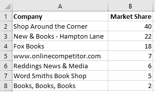
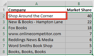
We will be using the same source data as before.  However, to keep things simple, we will assume that this data is already sorted (if you want to follow an example with unsorted data then follow the first part of last weeks’ post).

Creating the combo box

We will be using a combo box to select the row we wish to highlight.  A combo box is a type of input box which lets you select from a list (you’ll recognize it when you see it).  To create a combo box you will need the Developer Ribbon enabled.

Then click Developer -> Insert -> Combo Box (Form Control).

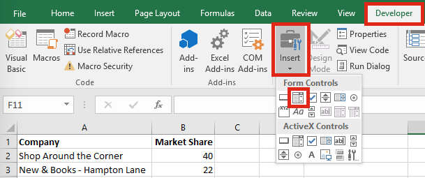
There is also a combo box in the ActiveX controls section, it is similar to the one we are using, but has a few different options.  For this example, we will stick with the Form Control version.

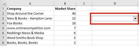
The mouse will become a + shape.  Click and drag a shape to represent the size and location where the combo box should be.  I have created a combo box as shown below.

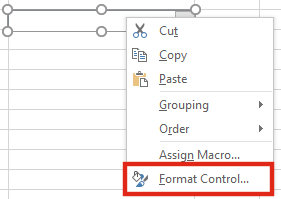
Next, right click on the combo box and select Format Control….

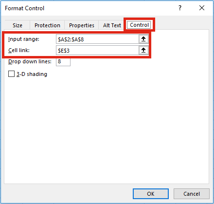
The Format Control window will appear.  There are two boxes to be completed:

• Input range – select the cells representing the list of companies.
• Cell link – select the cell to display the selected value.

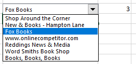
Now we can use the combo box to select values.  In the screenshot below I have selected Fox Books, this has a value of 3 as it is the 3rd item in the list.

Using INDEX to get the company name

The problem is that we want to match the company name of Fox Books, not the location in the list.  So, in Cell F3 we can use the INDEX function to obtain the company name.

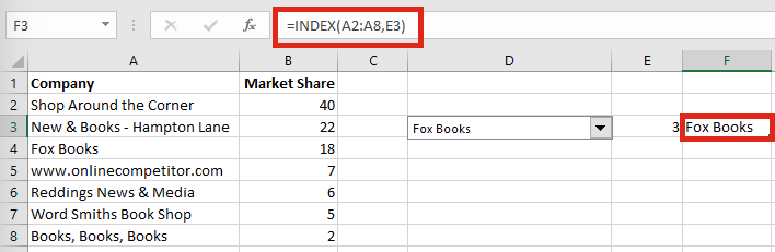
Cell F3 contains the following formula:

=INDEX(A2:A8,E3)

The formula is requesting the 3rd result (Cell E3) from the array of values (Cells A2-A8).  The result is Fox Books.

Highlighting the row

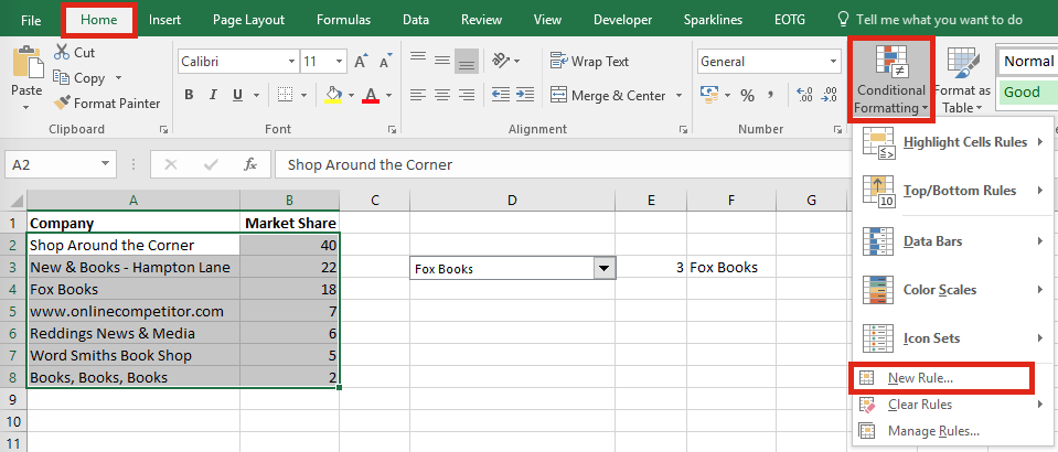
We will now use conditional formatting to highlight the row which matches the value in Cell F3.

Select the cells to be highlighted, click Home -> Conditional Formatting -> New Rules.

The New Formatting Rule window will open.  Select the last option in the list Use a formula to determine which cells to format.

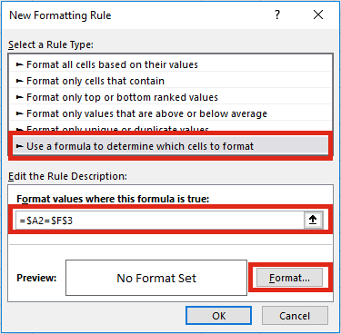
Next, we need to create our formula.   Our formula is:

=$A2=$F$3

The formula is written for the cell which is highlighted in the selected range (Cell A2 as shown below) but is applied to the whole range (Cells A2-B8).

The $ symbols are used in the formula to freeze the cell reference, just like normal in formulas.  Therefore, when Excel gets to Cell A3 it knows the formula should be as follows:

=$A3=$F$3

Equally, it will create the formula for Cells A4, A5 etc all the way down to A8.

Click Format, and select the formatting you wish.  I’ve chosen a mid-grey fill, so as not to over-power everything.  Click OK, OK again, then OK one more time.  You should now be back to your worksheet with the selected row highlighted.

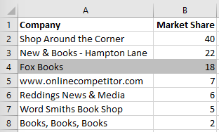
We can test the highlighting by changing the value in the combo box – Ta-Dah!  The highlighting now changes as the selection changes.  You just need to format it to look nice and you’ve now got an interactive table, which could be used on a dashboard.

---

What next?

Discover how you can automate your work with our Excel courses and tools.