How to create dynamic text in Excel (TEXT + Number Formats)

In a previous post, we looked at the ideal Excel number formats for accounting and finance. In each example, we formatted the cell values. However, there is another way to use these number formats; we can use them inside the TEXT function to generate custom headings and dynamic text. That’s what we are looking at in this post.

Table of Contents

• Understanding the TEXT function
• Syntax and arguments
• Simple example
• Different context: cells vs TEXT function
• Ignore the text format
• Reconsidering zero
• Alignment
• Colors
• Base format
• Applying format_text as cell value vs hardcoded
• Displaying units
• Symbols and decimal places
• Using number formats instead of the IF function
• Conclusion

Watch the Video

Watch on YouTube

Understanding the TEXT function

The purpose of the TEXT function is to convert a number into text using a specific number format.

Syntax and arguments

=TEXT(value, format_text)

• value – the number to convert to text
• format_text – a text string defining the number formatting to apply

Simple example

The following is a simple example to illustrate the TEXT function.

The formula in cell D4 is:

="Training costs for September were " &C4& "."

The number 5000 in cell C4 is included in the sentence, but there is no formatting.

We can do better than that. The formula in cell D5 includes the TEXT function:

="Training costs for September were " &TEXT(C5,"$#,##0") & "."

The $5,000 in C5 is still the same number but includes a currency symbol and a thousand separator. This is much easier to read.

To understand these number format codes, check out this post: Excel number formats for accounting & finance you NEED to know

To understand more about the text function: https://exceljet.net/functions/text-function

Different context: cells vs TEXT function

When applying number formats in the TEXT function, the display context differs from applying number formats to cells. Therefore we can simplify the basic number format.

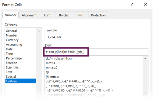
Let’s start with a common cell number format:

• Thousand separators
• Negative numbers in red with brackets
• Zero is a dash
• Correct number alignment (whitespace to the right)

#,##0_);[Red](#,##0);-_);@_)

When applied to cells, it displays positive, negative, zero, and text values as follows:

Ignore the text format

The 4th section of a number format code defines how text should display. However, the TEXT function already displays text. Therefore, the 4th section serves little purpose in the TEXT function. So, let’s ignore it.

Therefore, our example format changes from this:

#,##0_);[Red](#,##0);-_);@_)

To this:

#,##0_);[Red](#,##0);-_)

Reconsidering zero

The 3rd section of a number format code defines how zero values display. When used in a column of numbers, we may want to use a dash to represent a zero. But if we are concatenating with other text, the dash probably won’t look right. We are more likely to display zero as a number which is the default number format. Therefore, the zero format from the third position can also be ignored.

Our format changes again. From this:

#,##0_);[Red](#,##0);-_)

To this:

#,##0_);[Red](#,##0)

Alignment

When using number formats within a cell, we want negative numbers displayed in brackets/parentheses. To get the numbers to align correctly, we force whitespace to the right of positive numbers.

However, when using the TEXT function alignment of numbers is mostly irrelevant.

Our example format is simplified once again. From this:

#,##0_);[Red](#,##0)

To this:

#,##0;[Red](#,##0)

Colors

Finally, while colors work when formatting cells, they do not work within the TEXT function.

So, our format reduces one more time. From this:

#,##0_);[Red](#,##0)

This this:

#,##0;(#,##0)

Positive and zero values will display with at least one digit and a thousand separator. Negative numbers will display in brackets with at least one digit.

Base format

What started as the following, for a cell number format

#,##0_);[Red](#,##0);-_);@_)

Has been reduced to the following for a TEXT function number format:

#,##0;(#,##0)

Applying format_text as cell value vs hardcoded

Within the TEXT function, the format_text argument is a string. This can be hardcoded directly into the function, or it can be a cell-linked value.

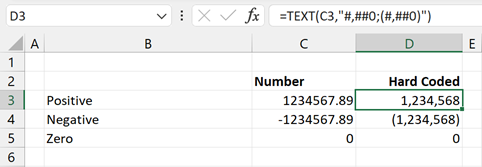
Hardcoded into function

The screenshot above shows the format_text applied as a hardcoded value.

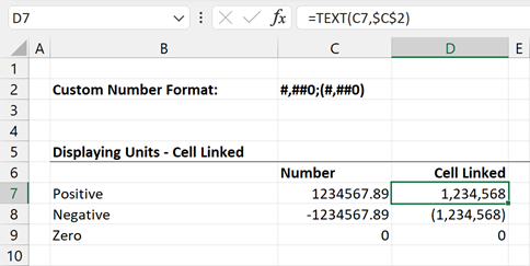
Cell driven

The screenshot above shows the format_text applied as a cell-linked value. The number format is included in cell C2.

This option creates more flexibility. However, we rarely, if ever, change these formats; therefore, I believe it is one scenario where it is acceptable to include hardcoded number formats in these functions.

Displaying units

Within the number format, we may wish to display units to provide more context to the numbers.

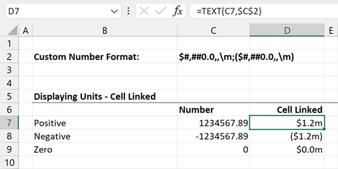
We can include currency symbols by including them within the format.

We can also include \k, \m, or \b to display numbers as thousands, millions, or billions.

When formatting numbers in this way, it is common to include commas and decimal places to display the required granularity. This prevents the need to divide a number to achieve the correct display format.

This number format also works with a hardcoded value in a TEXT function.

=TEXT(C17,"$#,##0.0,,\m;($#,##0.0,,\m)")

An alternative method uses double quotes around the letters. For the cell-linked method, this is no problem. The cell value would be:

$#,##0.0,,"m";($#,##0.0,,"m")

But for the hardcoded version we need to include additional double quotes to act as escape characters.

=TEXT(C14,”$#,##0.0,,””m””;($#,##0.0,,””m””)”)

We can also use CHAR(34) to represent a double quote character. Check out this post for more information about using double-quote characters in text strings: How to add double quotes in Excel formula.

Symbols and decimal places

Symbols and decimal places are the same for both methods. So we don’t need to apply any special treatment for those.

Using number formats instead of the IF function

A typical finance scenario may be to state if a movement is favorable or adverse to a prior period or budget.

We could generate the words favorable or adverse using an IF function.

The formula in cell D3 is:

=IF(C3>=0,"favorable","adverse")

In the screenshot above, C3 is positive, showing the word favorable.

However, we can achieve this directly with TEXT without an IF function.

The screenshot above shows the word favorable in cell E6 because the value in cell C6 is positive or zero. This value changes to adverse in cell E7 because cell C7 is negative.

The formula in cell F6 shows how we can use these TEXT functions to create sentences.

="There is a " & E6 & " variance of "& D6 & " to last month"

We can achieve the same favorable or adverse value from hardcoded formats.

The formula in cell E4 is:

=TEXT(C4,”””favorable””;””adverse”””)

With this method, the escape characters make the formula much harder to understand.

Conclusion

The custom number formats we use for cells can also be applied to the TEXT function. This provides a great way of adding dynamic commentary/insight into reports.

As the context differs from cell formatting, we may need to think differently about how we apply the number formats. We cannot use colors, but the other functionality is still available.

We’ve seen two ways to apply this: cell-linked or hard-coded values. Depending on the method we choose, we could encounter a few syntax issues. But we’ve covered these in this post, so hopefully won’t catch you out.

Related Posts:

• Excel number formats for accounting & finance you NEED to know
• Change number format based on a cells value
• How to add double quotes in Excel formula

---

What next?

Discover how you can automate your work with our Excel courses and tools.