How to calculate Power Query Percent of total or category

In this post, we look at how to calculate the percentage of a total in Power Query. But we will also take this one step further, to consider how to calculate the percent of a category.

In standard Excel, these calculations are simple because we are so used to the formulas to achieve this. For many, Power Query is still a newer tool, and it doesn’t operate in quite the same way. But once you’ve calculated a Power Query percentage of total, I think you will find is straightforward.

Table of Contents

• Power Query percent of total – quick answer
• Percent of total in Power Query
• Percent of category in Power Query
• How % of total works
• How % of category works
• Step 1
• Step 2
• Step 3
• Step 4
• Step 5
• Step 6
• Step 7
• Conclusion

Power Query percent of total – quick answer

The data in our example looks like this; it is a list of cities where a company has offices. Each office has a region and a headcount value.

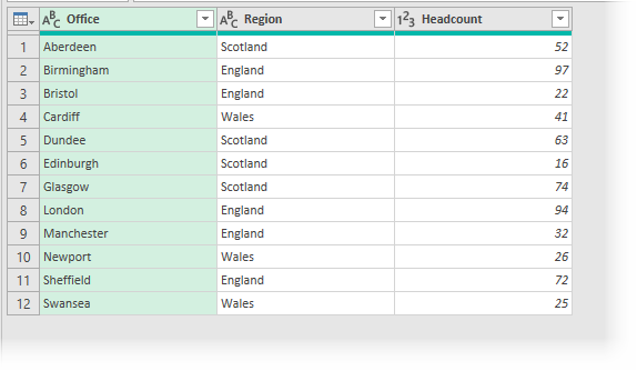
Our goal is to:

• Calculate the % of total headcount at each site
• Calculate the % of Region head count at each site

Percent of total in Power Query

To calculate the % of the total is reasonably straightforward. While the SUM function does not exist in Power Query, the List.Sum function does.

1. Within Power Query click Add Column > Custom Column
   
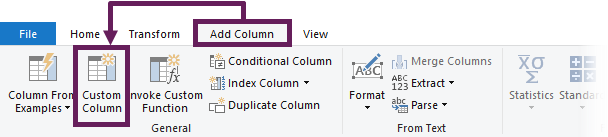
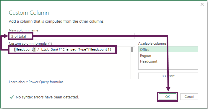
2. In the Custom Column dialog box enter the following formula: =[Headcount] / List.Sum(#”Changed Type”[Headcount])
3. Change the formula to fit your scenario:
   • [Headcount] is the name of the column for which you want to calculate the %
   • #”Changed Type” is the name of the step to be used as the source for the formula. Typically, this is the name of the previous step in the Advanced Editor window.
4. Give the custom column a useful name, such as % of total, then click OK.
   
5. The % of total column is now included in the preview window.
   
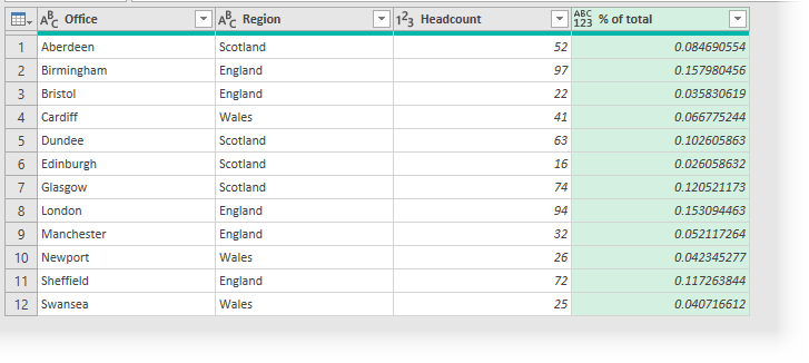
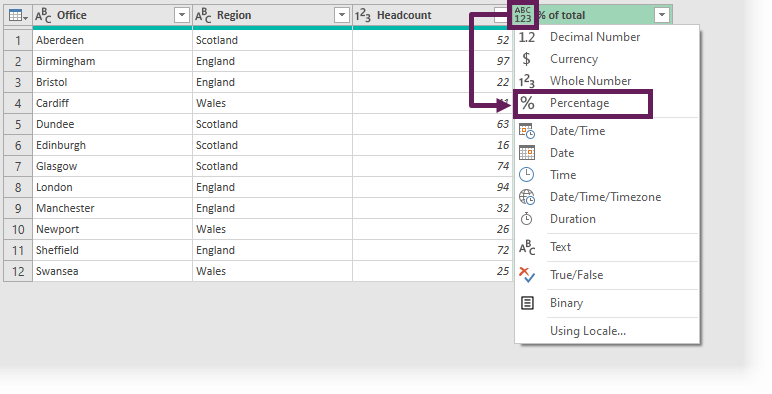
6. It doesn’t look like a percentage yet, so change the data type by clicking on the ABC123 button and selecting Percentage from the menu.
   

That’s it, here is the final table:

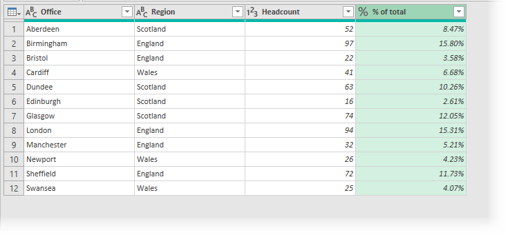
That wasn’t too bad, was it, eh? The solution was very similar to how we would do it in Excel. Keep reading to understand more about how this calculation works.

Percent of category in Power Query

To calculate the % of a category, it’s not quite as easy. Power Query does not have the equivalent of the SUMIF or SUMIFS functions, so we need to think differently. Instead, we create a transformation formula to achieve the same result.

1. Within Power Query click Add Column > Custom Column
   
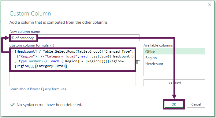
2. In the Custom Column dialog box enter the following formula:
   =[Headcount] / Table.SelectRows( Table.Group(#”Changed Type”, {“Region”}, {{“Category Total”, each List.Sum([Headcount]), type number}}) , each ([Region] = [Region])){[Region=[Region]]}[Category Total]
3. Change the formula to fit your scenario:
   • #”Changed Type” is the name of the step to be used as the source for the formula. Typically, this is the name of the previous step in the Advanced Editor window
   • [Region] or “Region” is the name of the column which contains the field to categorize by
   • [Headcount] is the name of the column for which you want to calculate the %
4. Give the custom column a useful name, such as % of category, then click OK.
   
5. The % of category column ins included in the preview window.
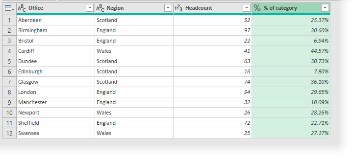
6. Finally, change the data type to percentage.

Here is the final table:

The process was similar to calculating the percent of a total, but the formula you pasted is much more complex. In the sections below, we’ll dig a bit deep to understand how it works. This will enable you to create this transformation for yourself.

How % of total works

Power Query, itself does not have a total row. This isn’t a problem, as the tool is intended for data manipulation, rather than presentation. But it does mean there is not a total row to divide by.

List.Sum is similar to Excel’s SUM function. The following M code uses that formula to calculate the total value for the Headcount column, using the #”Changed Type” step as its source.

List.Sum(#"Changed Type"[Headcount])

Having calculated the total, we just need to divide the number in each row of the headcount column by the result of the List.Sum function result.

=[Headcount] / List.Sum(#"Changed Type"[Headcount])

Pretty easy, right?

Learn more about the List.Sum function here: https://bioffthegrid.com/list-sum

How % of category works

Calculating the % of a category is a little tricky. We have seen this scenario previously when we looked at custom functions. While a custom function is an option, we can also achieve the result (and possibly easier) by nesting transformations into a single formula.

We will step through the transformations one-by-one so that we can understand how the technique works.

Step 1

Begin with the source table loaded into Power Query.

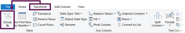
Step 2

Click Transform > Group By from the Power Query ribbon.

The Group By dialog box opens. Enter the following information:

• View: Basic
• Column: Region (i.e., the column which contains the category column)
• New column name: Any name you want. Given our data set, Total Region seems sensible
• Operation: Sum – the calculation we want to perform
• Column: Headcount – the column containing the numbers we want to perform the operation on

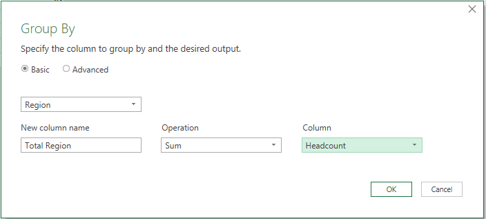
Click OK to close the dialog box.

Look at the formula bar at the top of the Preview Window (click View > Formula Bar if it is not visible). The M code for this step looks like this:

= Table.Group(#"Changed Type", {"Region"}, 
{{"Total Region", each List.Sum([Headcount]), type number}})

The Table.Group function is the M code which executes the Group By transformation. Learn more about the Table.Group function here: https://docs.microsoft.com/en-gb/powerquery-m/table-group

Step 3

Filter the category column to include a single value. I have selected Wales. Then click OK.

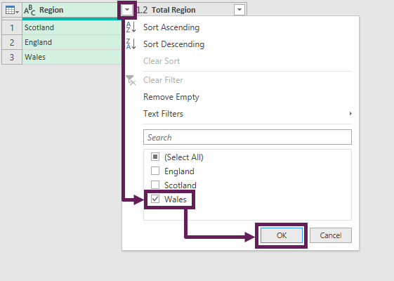
The M code for this step is:

= Table.SelectRows(#"Grouped Rows", each ([Region] = "Wales"))

The Table.SelectRows function is the M code that executes a column filter. Learn more about the Table.SelectRows function here: https://docs.microsoft.com/en-gb/powerquery-m/table-selectrows

Step 4

Now let’s combine the two transformations from Step 2 and Step 3 into a single formula.

#”Grouped Rows” is the reference to the step above. So, we just need to make two simple changes:

• Add the text before the step name to the beginning of the step above
• Add the text after the step name to the end of the step above

The M code now looks like this:

=Table.SelectRows(
Table.Group(#"Changed Type", {"Region"}, 
{{"Total Region", each List.Sum([Headcount]), type number}})
, each ([Region] = "Wales"))

The different sections are:

• The transformation from Step 2
• The code added from Step 3

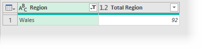
As the last step has now been added into the step above it is not longer required, we can delete the last step.

The preview window now only has one line of data.

Step 5

Right-click on the value within the Total Region column and select Drill Down from the menu.

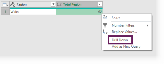
The M code for this step looks like this:

= #"Grouped Rows"{[Region="Wales"]}[Total Region]

Step 6

Now let’s add the code from step 5 into Step 4.

The M code now looks like this:

=Table.SelectRows(
Table.Group(#"Changed Type", {"Region"}, 
{{"Total Region", each List.Sum([Headcount]), type number}})
, each ([Region] = "Wales")){[Region="Wales"]}[Total Region]

The sections are:

• The transformation from Step 2
• The added code from Step 3
• The added code from Step 5

As the drill down has now been incorporated into the step above, we can delete the last step from the applied steps window.

Step 7

We now have all the transformations required, so it’s time to turn the formula into its own column.

1. Copy all the text for the combined formula from the Formula Bar.
2. Delete the step containing the formula from the Applied Steps list.
3. Click Add Column > Custom Column
4. Paste the copied text into the Custom Column dialog box.
   
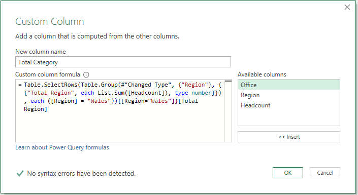
5. Replace each instance of “Wales” with [Region]. The code now looks like this: Obviously, you’ll adapt this to your scenario.
   =Table.SelectRows( Table.Group(#”Changed Type”, {“Region”}, {{“Total Region”, each List.Sum([Headcount]), type number}}) , each ([Region] = [Region])){[Region=[Region]]}[Total Region]
6. Finally, add the column to be divided to the start of the formula =[Headcount] / Table.SelectRows( Table.Group(#”Changed Type”, {“Region”}, {{“Total Region”, each List.Sum([Headcount]), type number}}) , each ([Region] = [Region])){[Region=[Region]]}[Total Region]

That’s it; we now have a % of the region for every row.

Conclusion

In this post, we focused on how to calculate the percentage of a total in Power Query and also the percentage of a category. Through this, we learned about the List.Sum function (which is similar to Excel’s SUM function) and also how to combine queries into a single transformation step. This is a great technique to achieve more advanced transformations.

Related posts:

• Introduction to Power Query
• How to use Power Query Group By to summarize data
• Power Query – Running Total

---

What next?

Discover how you can automate your work with our Excel courses and tools.

The Excel Academy