Have you ever had to sum the same cell across multiple sheets? This often occurs where information is held in numerous sheets in a consistent format. For example, it could be a monthly report with a tab for each month (see screenshot below as an example).
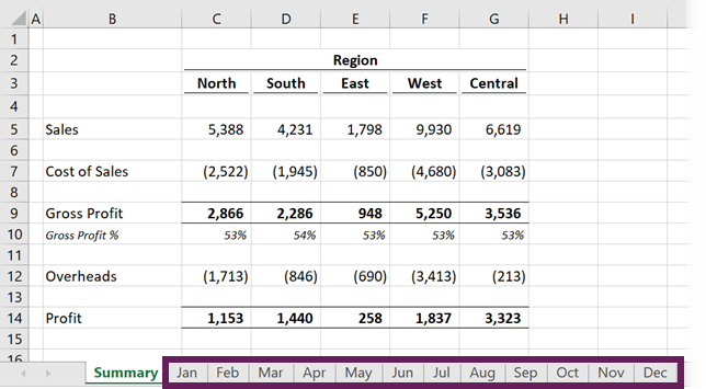
Table of Contents
Watch the video

I see many examples where the user has clicked the same cell on each sheet, putting a “+” symbol between each reference. If there are a lot of worksheets, it takes a while to click on them all. Also, if the sheet names are long, the formula starts to look quite unreadable. The screenshot below shows an example of this type of approach.
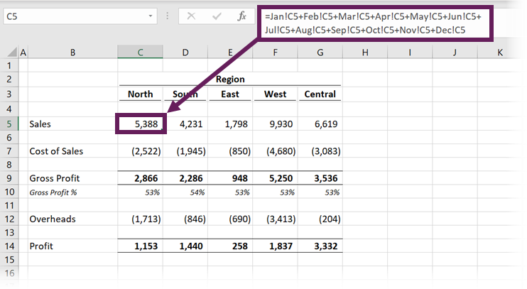
The formula in cell C5 is:
=Jan!C5+Feb!C5+Mar!C5+Apr!C5+May!C5+Jun!C5+
Jul!C5+Aug!C5+Sep!C5+Oct!C5+Nov!C5+Dec!C5
How do you know if you’ve clicked on every worksheet? What if you happened to miss one by accident? There is only one way to know – you’ve got to check it!
The chances are that you don’t need to do all that clicking. And just think about the time you will waste if there is a new tab to be added.
The good news is that there is another approach we can take that will enable us to sum across different sheets easily. I still remember the first time a work colleague showed me this trick; my jaw hit the ground in amazement. I thought he was an Excel genius. That’s why I’m sharing it here; by using this approach, you can look like an Excel genius to your work colleagues too 🙂
SUM across multiple sheets – basic
To sum the same cell across multiple sheets of a workbook, we can use the following formula structure:
=SUM('FirstSheet:LastSheet'!A1)
- Replace FirstSheet and LastSheet with the worksheet names you wish to sum between. If your worksheet names contain spaces, or are the name of a range (e.g., Q1 could be the name of a sheet or a cell reference ), then single quotes ( ‘ ) are required around the sheet names. If not, the single quotes can be left out.
- Replace A1 with the cell reference you wish to use
With this beautiful little formula, we can see all the worksheets included in the calculation just by looking at the tabs at the bottom. Take a look at the screenshot below. All the tabs from Jan to Dec are included in the calculation.
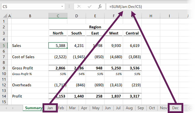
The formula in cell C5 is:
=SUM(Jan:Dec!C5)
SUM across multiple sheets – dynamic
We can change this to be more dynamic, making it even easier to use. Instead of using the names of the first and last tabs, we can create two blank sheets to act as bookends for our calculation.
Take a look at the screenshot below. The Start and End sheets are blank. By dragging sheets in and out of the Start and End bookends, we can sum almost anything we want.
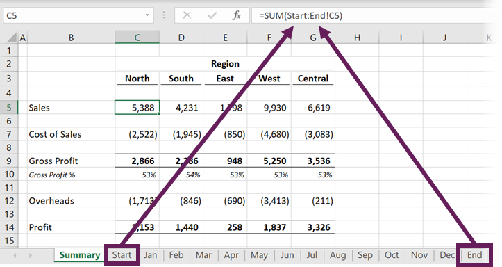
The formula in cell C5 is
=SUM(Start:End!C5)
We can also create sub-calculations. For example, we could add quarters as interim bookends too. There is the added advantage that the tabs also serve as helpful presentation dividers. The example below shows the calculation of just Jan, Feb, and Mar sheets.
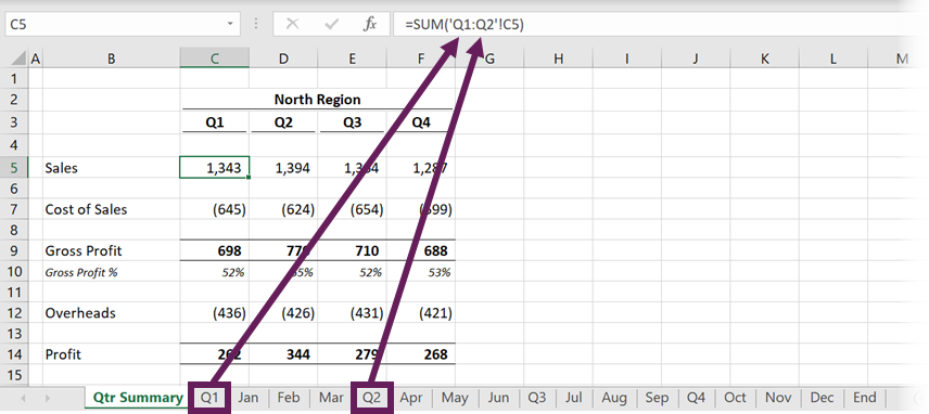
The formula in cell C5 is:
=SUM('Q1:Q2'!C5)
Excel could mistake Q1 and Q2 as cell references; therefore, adding single quotes around the sheet names is essential.
Which other formulas does this work for?
This approach doesn’t just work for the SUM function. Here is a list of all the functions for which this trick works.
| Basic Calculations SUM AVERAGE AVERAGEA PRODUCT | Counting COUNT COUNTA | Min & Max MAX MAXA MIN MINA | Standard deviation STDEV STDEVA STDEVP STDEVPA | Variance VAR VARA VARP VARPA |
The drawbacks
There are a few things to be aware of:
- All the sheets must be in a consistent layout and must stay that way. If one worksheet changes, the formula many not sum the correct cells.
- Usually, formula cell references move automatically when new rows or columns are inserted. This formula does not work like that. It will only move if you select all the sheets and then insert a row or column into all of those sheets at the same time.
- Any sheets which are between the two tabs are included within the calculation. Therefore, even though we cannot see them, hidden sheets are also included in the result.
Discover how you can automate your work with our Excel courses and tools.
The Excel Academy

Make working late a thing of the past.
The Excel Academy is Excel training for professionals who want to save time.
Your explanation is great and your video is really helpful. However, I am having trouble getting this to work. I am following your instructions to the letter. I watched many other tutorials which are similar and I can’t figure out the problem. I just keep getting the syntax error in the cell that I’m trying to total “####”. I’ve noticed a few subtle differences in tutorials and have tried everything. Could it have something to do with the fact that I’m using the free version on Excel and not the pay version?
To my knowledge, this has been around in Excel since version 1, which was in the mid-1980’s. I’ve tested it in Excel Online and it works.
It’s not just a matter of making the column wider is it?
What do you mean by “free version of Excel”? Do you mean Excel Online?
it’s not working – I followed all the steps using Google Sheets but it’s giving an error 🙁
Google Sheets is not the same as Excel, so the same techniques may not work.