Power Query: Get data when sheet/Table names change (2 ways)

Recently, one of our academy members asked how to get data from an Excel workbook when sheet or Table names change. By default, Power Query uses names to filter down to the correct data. Therefore, if the sheet or Table names change every time a report downloads, that will cause errors.

We don’t want to update the query, and we don’t want to edit the workbook. So, instead of getting a Table or sheet by name, how can we get it by position? That’s the problem we are solving in this post.

Table of Contents

• Understanding the Navigation Step
• The Solution
• User Interface Method
• Writing M code
• Conclusion

Watch the Video

Watch the video on YouTube

Understanding the Navigation Step

Let’s start by understanding what Power Query does by default.

To get a Table or sheet into Power Query, we click Data > Get Data > From File > From Excel Workbook.

Next, we navigate to the Excel workbook, then click Import.

In the Navigator window, we select the individual sheet or Table and click Transform Data.

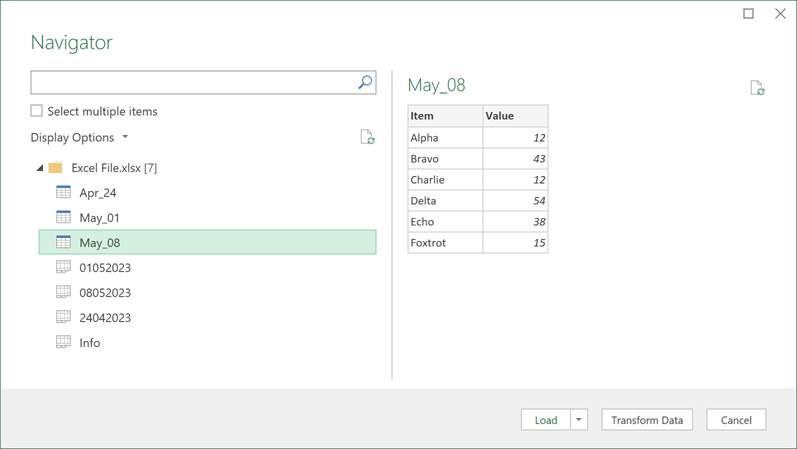
This creates the Navigation step in the Applied Steps window. Depending on your settings, you may have Promoted Headers and/or Changed Type steps too.

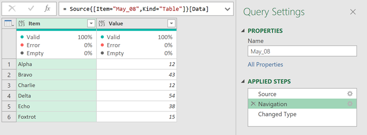
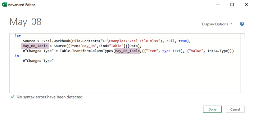
As a side note, Navigation is not actually the name of the step. Looking at the Advanced Editor reveals the real name of the step. In our example, the step is called May_08_Table.

We had selected the sheet called 08052023; the step would be called 08052023_Sheet in the advanced editor.

Whether we look at the code in the Advanced Editor or the Formula Bar, we can see the following formula for the Navigation step.

= Source{[Item="May_08",Kind="Table"]}[Data]

What does this code do?

• Source – The name of the previous step.
• {[Name=”myTable”, Kind=”Table”]}
  • This filters the record by Name and Kind.
  • The filters must always leave a single record remaining for this method to work.
• [Data] – This is the name of the column to expand.

If we only filter by Kind, this may generate an error where there are multiple Tables or Sheets. In our example, the code below creates an error because there are three Tables in the workbook.

= Source{[Kind="Table"]}[Data]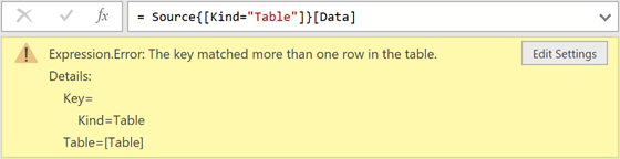

The Solution

So, to filter to a specified Table or sheet by position, we need to find an alternative approach that achieves the same result.

Let’s look at this in two ways (1) User Interface (2) Writing M code

User Interface Method

If we only want to use the user interface, we can apply the following steps.

1. Delete the Navigation step (also delete Promoted Headers and Changed Type if they were automatically applied).
2. Filter the Kind column to Sheet or Table for your scenario.
3. Select the Data column, then click Home > Remove Columns (drop-down) > Remove Other Columns
4. Click on the word Table in the Data column for the position we want to drill into.

That’s it. We’re done.

Let’s take a look at the M code in the Advanced Editor.

let
    Source = Excel.Workbook(File.Contents("C:\Examples\Excel File.xlsx"), null, true),
    #"Filtered Rows" = Table.SelectRows(Source, each ([Kind] = "Table")),
    #"Removed Other Columns" = Table.SelectColumns(#"Filtered Rows",{"Data"}),
    Data = #"Removed Other Columns"{2}[Data]
in
    Data

Perfect. No specific Table or sheet names are included in the code; only the row number of the sheet or Table. So if the names change, it’s not a problem; itstill operates correctly.

The key piece of code is {2}. It declares that we want the third Table. If we replaced it with {0}, it would be the first Table, the second Table would be {1} etc.

Now, you might wonder in which order the worksheet objects appear. Power Query lists the Sheets in the same order as the workbook. First, Sheets left to right, then Tables left to right. Therefore provided we filter by Kind initially, we should be able to get the nth sheet or Table from a workbook.

The code shows 3 steps to achieve what Navigation did in 1. This is not a big problem; the code is still efficient and will execute quickly. But if you like your M code to be as short as possible, the M code version below may be a better option.

Writing M code

If we are willing to venture into writing M code, we can combine the code from the sections above into a single line. We just need 3 elements.

• Filter the Table with Table.SelectRows() function
• Get the Nth position from the table. {2} in our example
• Drill into the [Data] column

To achieve that, delete all the steps except Source. Then, click the fx icon next to the formula bar to create a new step. Enter the following:

= Table.SelectRows(Source, each ([Kind] = "Table")){2}[Data]

If you look closely, you will notice this is an amalgamation of other code sections created by Power Query for the User Interface method above.

Now we benefit from a single step to select a Table or sheet by position.

Conclusion

In this post, we have seen how to filter by position in Power Query to extract a Table or sheet when their names change.

The techniques are not restricted to this scenario but are helpful for many other tricky PQ situations.

Related posts:

• Rename columns in Power Query when names change
• How to remove spaces in Power Query
• Introduction to Power Query

---

What next?

Discover how you can automate your work with our Excel courses and tools.

The Excel Academy