Rename columns in Power Query when names change

Power Query is great for extracting data from a source, reshaping it, then loading it into Excel. A standard part of the transformation process involves Power Query using column headers to reference each column. When the column headers change in the source data, it gives us a big problem.

Recently, my friend, Celia Alves released a YouTube video giving her solution to this problem. There is so much good stuff in that video showing how to use M code formulas and list techniques. You should definitely check out her video her solution: https://youtu.be/wSwXyfaXQgU. So, in this post, I want to share two ways to rename columns in Power Query when the column names change.

I’ve got two approaches that are a little different to Celia’s, so I thought I would post my solutions to this common problem in the interest of sharing other techniques.

Table of Contents

• The problem
• Solution #1 – Using only the User Interface
• Load the data in Power Query
• Remove Promote Headers & Changed Type
• Delete top 3 rows
• Promote headers
• Unpivot other columns
• Add an index/modulo column
• Replace the values
• Delete the Attribute column
• Pivot the header column
• Apply Changed Type
• Close and Load into Excel
• Refresh the query
• Solution #2 – Editing M Code
• Initial transformations
• Rename the columns manually
• Change the M code formula
• Final transformations
• Conclusion

Watch the video

Watch the video on YouTube.

The problem

Let’s assume we receive the following file each week:

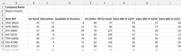
It doesn’t look too tricky to transform in Power Query. But it becomes tricky the following week when we receive an updated version of the file:

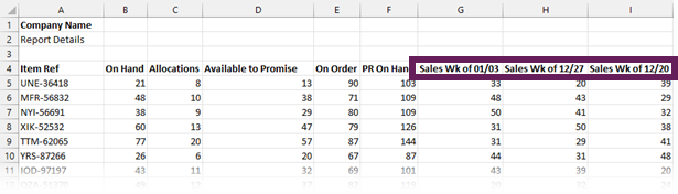
The headings for the last 3 columns have changed. Therefore, when we refresh the query, we get the following error:

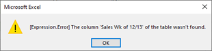
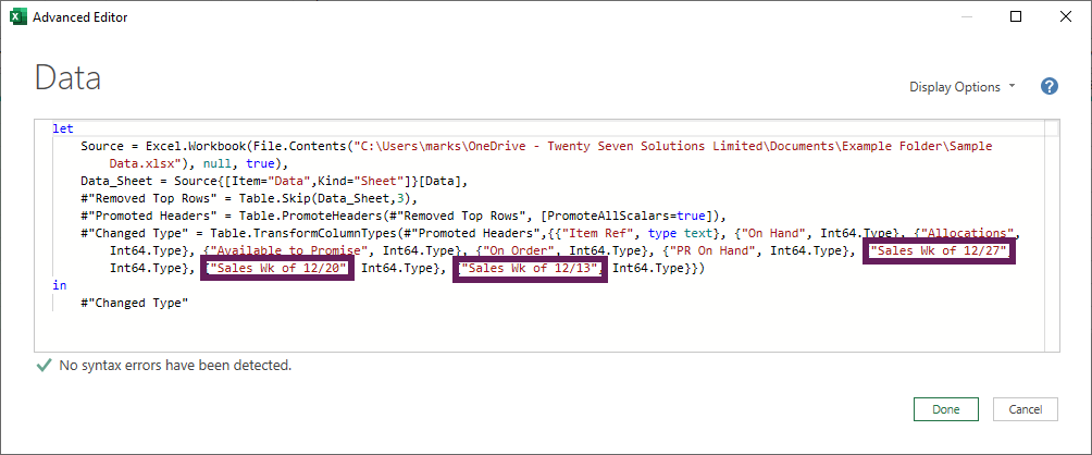
The problem with the query is the column headers are explicitly stated in the M code during the Changed Type step.

So, how can we rename columns in Power Query when names change? Let’s find out.

Solution #1 – Using only the User Interface

The first solution is based entirely on the user interface; there are no coding requirements. There are quite a few steps, but hopefully, nothing too tricky.

Load the data in Power Query

To load the example data into Power Query:

1. In the ribbon, click Data> Get Data > From File > From Workbook
   
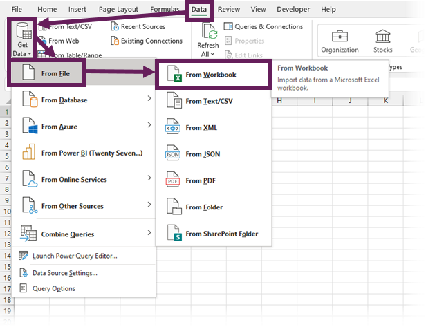
2. Navigate to the file location and click Import
3. The Navigator window opens, select Data and click the Transform Data button
   

Remove Promote Headers & Changed Type

If you have the default Power Query setup, then your preview window will look like this:

At present, we don’t need the Promoted Headers or Changed Type step, so delete those steps by clicking on the cross next to each.

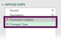
Note: If you have changed your default Power Query setup, you may not need to remove these steps.

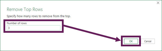
Delete top 3 rows

The top 3 rows are not part of the data set, so we can remove those:

1. Click Home > Remove Rows (dropdown) > Remove Top Rows
   
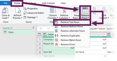
2. Enter 3 into the Remove Top Rows dialog box and click OK
   

Promote headers

Now we can promote headers by clicking Home > Use First Rows as Header

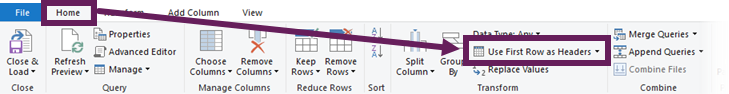
If the Changed Type step automatically appears, delete it. 

So far, so good; no column names have been included in the code.

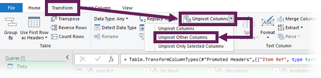
Unpivot other columns

Next, we want to unpivot those columns with the names that change.

1. Select all the columns with names that will not change; in this example, that is columns from Item Ref to PR on Hand.
2. Click Transform > Unpivot Columns (dropdown) > Unpivot Other Columns
   

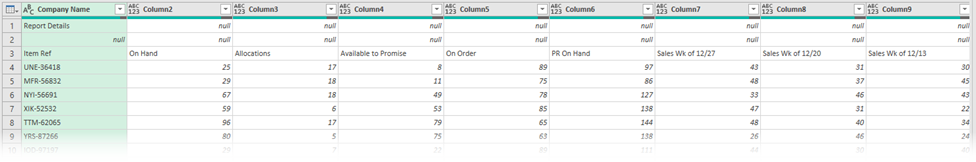
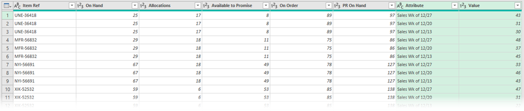
The preview window data now looks like this. The Attribute column now contains the names of the columns.

Add an index/modulo column

As there were 3 columns with names that change, we want to create a reoccurring numbering of 0 to 2 against each of those items. That might seem strange, but it will all become clear once it’s completed:

• From the ribbon, click Add Column > Index Column (dropdown) > From 0
  
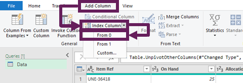
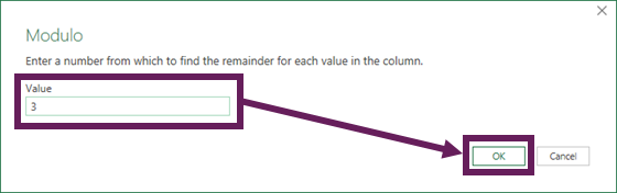
• With the Index column selected click Transform > Standard (dropdown) > Modulo
  
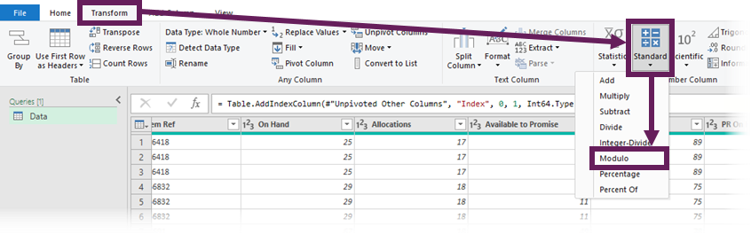
• As there are 3 columns, enter 3 into the Modulo window and click OK.
  

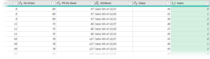
The preview window now looks like this. Notice the Index column has values 0, 1, 2 repeating

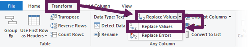
Replace the values

Then we will replace each number with the name of the header we want to use.

1. Change the data type of the Index column to Text, by clicking on the data type icon and selecting Text from the menu.
   
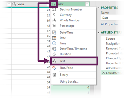
2. Transform > Replace Values (dropdown) > Replace Values
   
3. In the Replace Values window, apply the following parameters
   Value To Find: 0
   Replace With: Last Week Sales
   Then click OK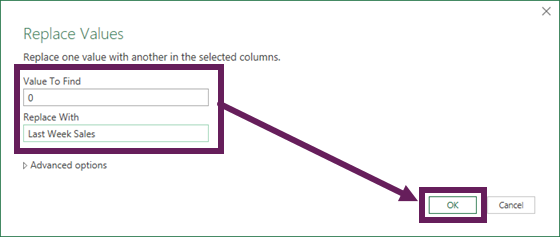
   
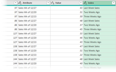
4. Repeat steps 2 and 3 for the other columns:
   • 1 is replaced with Two Weeks Ago
   • 2 is replaced with Three Weeks Ago

Delete the Attribute column

We have no further use for the Attribute column created during the Unpivot process.

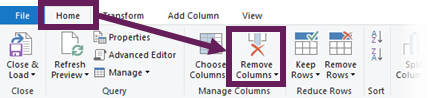
Select the Attribute column and click Home > Remove Column

Pivot the header column

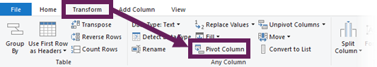
The Index column now contains the new headers we want to apply, so let’s Pivot on that column to create the new headers.

1. With the Index column selected, click Transform > Pivot
   
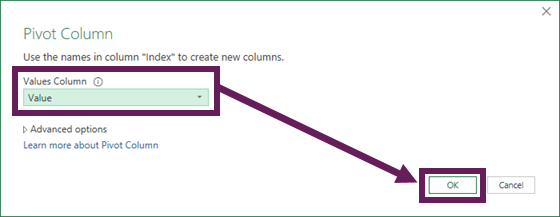
2. In the Pivot Column window, select Values from the dropdown box (as that contains the numeric values for each column). Then click OK.
   

Apply Changed Type

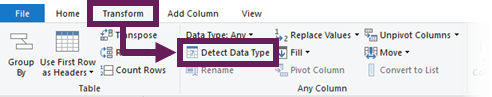
We can now apply the Changed Type step. I would generally recommend looking at each column individually and deciding on the data type, but for this illustration, we will let Power Query choose the default type.

Select all the columns and click Transform > Detect Data Type

Close and Load into Excel

Finally, we can load the table into Excel.

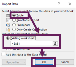
1. Click Home > Close & Load (dropdown) > Close & Load To…
   
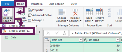
2. From the Import Data dialog box, select a Table in the existing Worksheet in cell A1, then click OK.
   

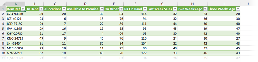
This is what Excel looks like with the new column names.

Refresh the query

OK, now let’s assume we’ve got some updated data.

• Delete the Sample Data.xlsx file
• Rename Sample Data – New.xlsx to be Sample Data.xlsx
• In Excel, click Data > Refresh All

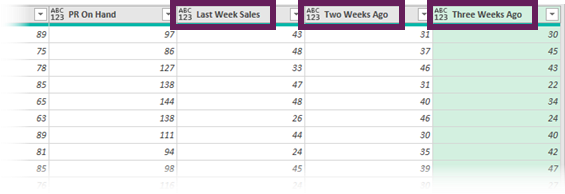
The query now refreshes and… Ta-Dah! The data below loads!

Amazing!!! The query refreshes with no errors 😀.

Solution #2 – Editing M Code

OK, now it’s time to look into another solution. This solution is much easier, but you have to feel a little confident editing the M formulas to get this right.

Initial transformations

Follow the steps in Solution #1 until the end of the Promote Headers step, then come back here.

Rename the columns manually

Go ahead and just double-click on each of the columns you wish to rename and change them.

The column names are included in the M code. Isn’t this precisely what we said we didn’t want to do!!! Yes, it is. But just wait; it’s all about to come together.

Change the M code formula

M code is not the most forgiving of languages; you need to make the syntax changes exactly as stated below (including the correct upper and lower case).

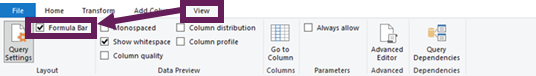
If the formula bar is not visible, click View > Formula Bar

Select the Rename Column step and make the following changes in the formula bar. Change the highlighted text from this (the code has been wrapped for the ease of reading):

= Table.RenameColumns(#"Promoted Headers",{{
"Sales Wk of 12/27", "Last Week Sales"}, 
{"Sales Wk of 12/20", "Two Weeks Ago"}, 
{"Sales Wk of 12/13", "Three Weeks Ago"}})

to this:

= Table.RenameColumns(#"Promoted Headers",{
{Table.ColumnNames(#"Promoted Headers"){6}, "Last Week Sales"}, 
{Table.ColumnNames(#"Promoted Headers"){7}, "Two Weeks Ago"}, 
{Table.ColumnNames(#"Promoted Headers"){8}, "Three Weeks Ago"}})

So, rather than changing a column based on its name, we are changing it based on its position.

Note: “Sales Wk of 12/27” is column 6 in Power Query even though it is the 7th column. Power Query starts counting at zero, so while it’s the 7th column, the column number for Power Query is always 1 lower.

Final transformations

Now pick up Solution #1at the Apply Changes step, then work through to the end.

Once again, we have changed column names even when the source data changes.

Conclusion

This post proves that there are multiple ways of solving the same problem in Power Query. For example, Celia’s approach and my approaches above are all completely different, yet they achieve the same result.

Which method you use is up to you, but in comparing all three approaches, I hope you’ve learned a lot about using Power Query to solve problems.

---

What next?

Discover how you can automate your work with our Excel courses and tools.