How to FILTER by a list in Excel (including multiple lists)

A few weeks back, I wrote a post about how to filter by a list in Power Query. It didn’t take long for somebody to ask if the same is possible in Excel. The answer is, YES! So, that’s what we are looking at in this post: how to use Excel’s FILTER function based on a list.

Note: The solution in this post only works in Excel 2021 and Excel 365.

Table of Contents

• Understanding the FILTER function
• Calculating the TRUE/FALSE value
• FILTER based on a list
• FILTER by items NOT in the list
• FILTER based on multiple lists
• And condition (included in all lists)
• Or condition (included in any lists)
• Conclusion

Watch the video

Watch on YouTube

Understanding the FILTER function

Let’s start by looking at the FILTER function. FILTER has a simple syntax with just three arguments:

=FILTER(array, include, [if_empty])

• array: The range of cells, or array of values to filter.
• include: An array of TRUE/FALSE results, where only the TRUE values are retained in the filter.
• [if_empty]: The value to display if no rows are returned.
  

The include argument is where we need to focus our attention for the current requirements.

For each row of the source data, there needs to be a calculation that returns TRUE or FALSE. Only the TRUE values are retained in the FILTER result.

Therefore, the critical question is: How can we create a TRUE/FALSE result for each item? Let’s find out.

Want to know more about the FILTER function? Check out this post: FILTER function in Excel (How to + 8 Examples)

Calculating the TRUE/FALSE value

To calculate TRUE or FALSE, we could use the COUNTIFS function:

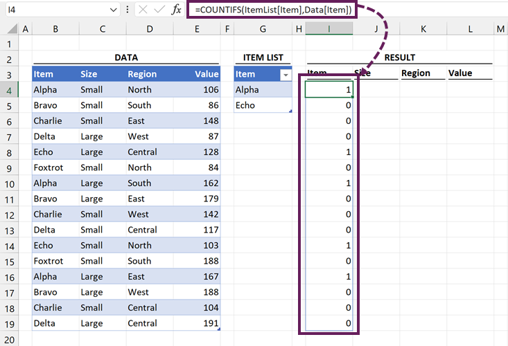
The formula in cell I4 is:

=COUNTIFS(ItemList[Item],Data[Item])

This is taking the values in the ItemList table and counting how many times they appear for each row of the Data table. This function uses dynamic arrays and spills the results.

You might be thinking that they are not TRUE or FALSE values but are 0’s and 1’s.

But the great thing about Excel is that 0 is deemed to be FALSE, and any other values are treated as TRUE. So, for Excel, this is the same as a TRUE/FALSE list. Which means we can use this inside the include argument.

Want to know more about COUNTIFS? Check out this post: https://exceljet.net/functions/countifs-function

FILTER based on a list

OK, now it’s time to add the FILTER function, using the COUNTIFS as the include argument.

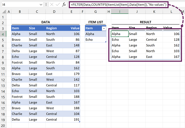
The formula in cell I4 is:

=FILTER(Data,COUNTIFS(ItemList[Item],Data[Item]),"No values")

The previous COUNTIFS formula is highlighted in bold.

Only the items from the Data table where the COUNTIFS calculates to 1 or more are retained.

FILTER by items NOT in the list

To filter by items not in the list, we wrap the COUNTIFS in the NOT function.

=FILTER(Data,NOT(COUNTIFS(ItemList[Item],Data[Item])),”No values”)

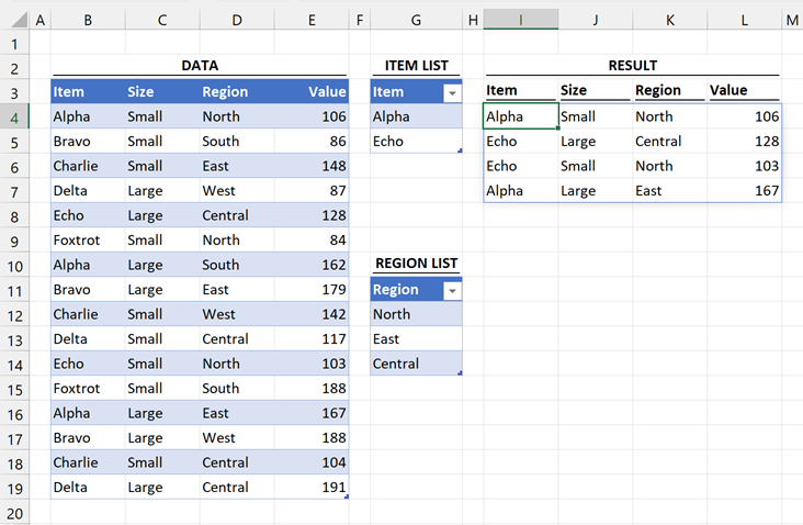
FILTER based on multiple lists

I know somebody will ask this, so I might as well answer it here.

Yes, using this method we can filter by multiple lists. We just add more COUNTIFS into the include argument.

And condition (included in all lists)

If we want items that appear in multiple lists:

• Use an asterisk ( * ) between each COUNTIFS
• Wrap all the COUNTIFS in the include argument in brackets

The formula in Cell I4 is:

=FILTER(Data,(COUNTIFS(ItemList[Item],Data[Item])*COUNTIFS(RegionList[Region],Data[Region])),"No values")

Notice the * symbol between the COUNTIFS. The items included in both the ItemList and RegionList are retained by the FILTER result.

Or condition (included in any lists)

Alternatively, to retain items that appear in any list:

• Use a plus ( + ) between each COUNTIFS
• Wrap all the COUNTIFS in the include argument in brackets,

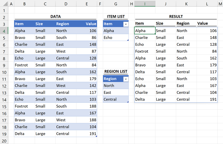
The formula in Cell I4 is:

=FILTER(Data,(COUNTIFS(ItemList[Item],Data[Item])+COUNTIFS(RegionList[Region],Data[Region])),"No values")

Notice the + symbol between the COUNTIFS. Items included in either the ItemList or RegionList are retained by the FILTER result.

Conclusion

In this post, we’ve seen how to break down the formula logic of the FILTER function. Through this, we were able to filter by a list in Excel using FILTER and COUNTIFS. We also took this further for and / or logic to filter by multiple lists.

---

What next?

Discover how you can automate your work with our Excel courses and tools.