Data comes in all shapes and sizes, and since Excel is not a database, we face those shapes and sizes on a daily basis. One advantage of Tables in Excel is that they force us to apply some standards to our data structure, such as:
- There can only be one header row
- The headers must be unique.
But even with these standards, we find data is often in a partly presentational format. Look at the example below; here the columns are shown in time order. This is what I mean by “a partly presentational format”.
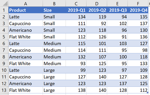
This isn’t the ideal format for computers to process data, but it is how our brains think, so often spreadsheets are presented in this way. However, this creates a problem when we want to provide the user with the ability to choose which column to use in Table. So what can we do?
Let’s work through some formula examples to dynamically select a column to use inside a SUMIFS function. The three methods we will use are:
- INDIRECT
- INDEX / MATCH
- SUMPRODUCT
The Table in our example is called tblSales, which is referred to throughout the rest of the post.
Dynamic column selection with INDIRECT
The INDIRECT function is used to convert a text string into a range, for use inside another formula. As a simple example, the following formula will return the value in Cell B4.
=INDIRECT("B4")
The “B4” in the formula above is not a Cell reference; it is surrounded by double quotation marks, so it is a text string. The Structured References used with Tables can also be used as a text string within the INDIRECT function.
The structured reference for the 2019-Q3 column of the tblSales Table would be:
tblSales[2019-Q3]
To use this inside the INDIRECT function would be as follows:
INDIRECT("tblSales[2019-Q3]")
Now it’s time to make this dynamic. If the text 2019-Q3 were contained within another cell it could be inserted into the INDIRECT function as follows (I’m assuming Cell I4 contains the text 2019-Q3).
INDIRECT("tblSales["&I4&"]")
The & is used to join the text with the value in Cell I4 to create a single text string (the technical term for this is to concatenate).
We can now insert the INDIRECT function into the SUMIFS function:
=SUMIFS(INDIRECT("tblSales["&I4&"]"),tblSales[Product],I2)
This is shown below in Cell I9.
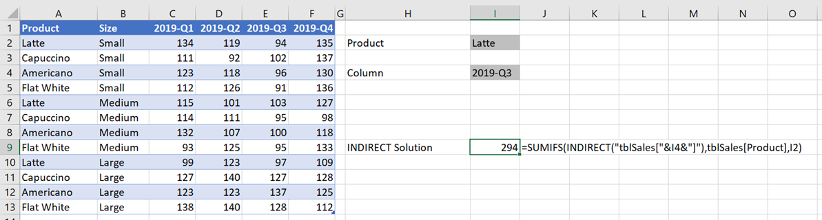
The value in Cell I4 can be changed to select any column, therefore the SUMIFS function can now be changed to any column dynamically.
Before you get too excited; the INDIRECT function has one big issue – it’s a volatile function. Normally, Excel only recalculates a formula when any preceding cell changes. This not true of volatile functions, they and any dependent cells recalculate with every change. Therefore, if you get a lot of volatile formulas, or where one is used early in the calculation chain, they can drastically slow down calculation times.
Dynamic column selection with INDEX / MATCH
INDEX / MATCH can also be used to dynamically select a column from a Table, and has the advantage of not being volatile. INDEX / MATCH will only recalculate when preceding cells change. However, it more complicated to apply and harder for an average user to understand.
INDEX / MATCH has a superpower which most users are unaware of… it can return an entire column or row of results. Therefore with this formula combination we can insert the dynamically selected column into the SUMIFS.
MATCH Function
MATCH returns the position of a lookup value from a range. So if we search for 2019-Q3 from the header section of the Table, it should return 5, as it is the 5th cell within the header.
=MATCH("2019-Q3",tblSales[#Headers],0)
tblSales[#Headers] refers to the header row of the Table.
INDEX Function
INDEX is used to return a value (or values) from a one or two-dimensional range. As a simple example, the following would return the 2nd row and 5th column from the Table.
=INDEX(tblSales,2,5)
By using tblSales, we are referencing the body of the Table. It does not include the Headers or the Totals.
When using the INDEX function, if the row or column number is given a value of 0 or excluded, it will return the entire row or column. Therefore the following will return the whole 5th column from the Table.
INDEX(tblSales,0,5)
Or the alternative is to exclude the 0; please note the comma must remain,
INDEX(tblSales,,5)
INDEX & MATCH joined
Let’s now join these two functions together:
=INDEX(tblSales,0,MATCH("2019-Q3",tblSales[#Headers],0))
The MATCH function in our example will return 5, therefore the INDEX function will return all the values in the 5th column. We can include this within the SUMIFS function so that only the values from the 2019-Q3 column are included within the calculation.
=SUMIFS(INDEX(tblSales,,MATCH("2019-Q3",tblSales[#Headers],0)),tblSales[Product],I2)
Just as we did with INDIRECT, we can reference a cell to make it more dynamic for a user.
=SUMIFS(INDEX(tblSales,,MATCH(I4,tblSales[#Headers],0)),tblSales[Product],I2)
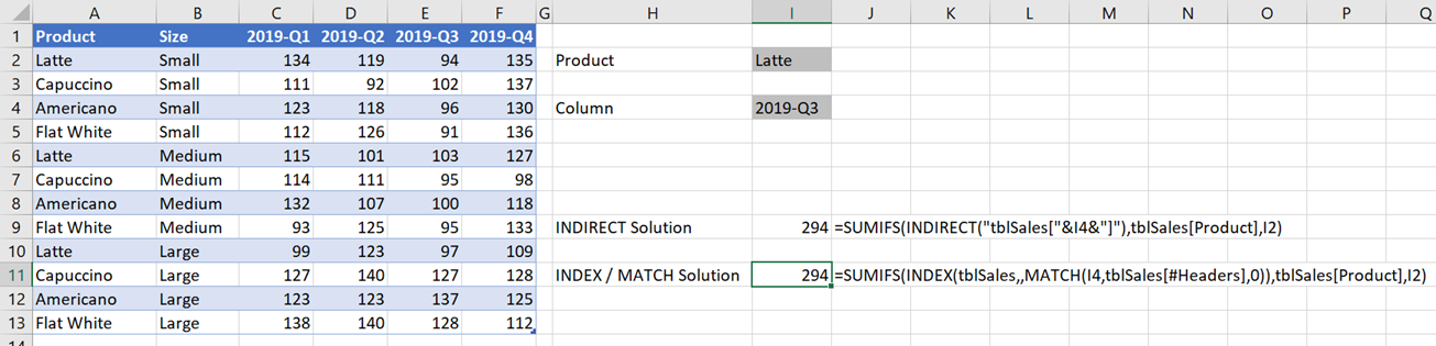
The value in Cell I4 determines which column do use within the SUMIFS function.
This is clearly a more complicated solution than INDIRECT, however being non-volatile makes is a better solution when dealing with large datasets.
SUMPRODUCT the ultimate weapon
But what if we want to sum multiple columns? Good question. To do that we need to leave the comforts of SUMIFS behind and head towards SUMPRODUCT.
SUMPRODUCT multiplies multiple ranges together and returns the result. Multiplication may not seem like the obvious solution to our problem, but trust me, it is.
The example below shows to sum the Lattes from 2019-Q2 or 2019-Q3.
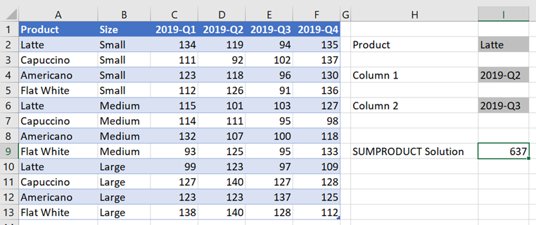
The formula in Cell I9 is:
=SUMPRODUCT((tblSales[[2019-Q1]:[2019-Q4]])*(tblSales[Product]=I2)*
(tblSales[[#Headers],[2019-Q1]:[2019-Q4]]>=I4)*(tblSales[[#Headers],[2019-Q1]:[2019-Q4]]<=I6))
Wow look at that, it’s so big that it needs multiple lines. As this is not a post about SUMPRODUCT, I will just highlight a few key points to illustrate the point.
The following identifies the cells which are greater than or equal to than 2019-Q2 (the value in Cell I4) and less than or equal to 2019-Q3 (the value in Cell I6).
(tblSales[[#Headers],[2019-Q1]:[2019-Q4]]>=I4)*(tblSales[[#Headers],[2019-Q1]:[2019-Q4]]<=I6))
Next we multiply to find which items are Latte’s
(tblSales[Product]=I2)*
(tblSales[[#Headers],[2019-Q1]:[2019-Q4]]>=I4)*(tblSales[[#Headers],[2019-Q1]:[2019-Q4]]<=I6)
Each cell which meets all the criteria has a value of 1, while the remaining cells have a value of 0. If we multiply that by the values in the table, only the 1’s will return a positive value.
=SUMPRODUCT((tblSales[[2019-Q1]:[2019-Q4]])*(tblSales[Product]=I2)*
(tblSales[[#Headers],[2019-Q1]:[2019-Q4]]>=I4)*(tblSales[[#Headers],[2019-Q1]:[2019-Q4]]<=I6))
Adding all these together provides the result of 637 in Cell I9.
SUMPRODUCT is clearly a very flexible function which can be used to sum values in two dimensions.
Conclusion
If SUMPRODUCT is so good why should we bother with INDIRECT or INDEX? It all comes down to the speed of calculation.
SUMPRODUCT is powerful but exceptionally slow, therefore if a single column result is sufficient, then INDEX / MATCH or INDIRECT will be much faster. And with INDIRECT being a volatile function, it makes INDEX MATCH the best option to use.
Discover how you can automate your work with our Excel courses and tools.
The Excel Academy

Make working late a thing of the past.
The Excel Academy is Excel training for professionals who want to save time.
Thanks it was really helpful. It opened my eyes I was searching for dynamic apply formula in the column but now I am on a right track
In case you’re looking for a solution after about the middle of 2023, there’s a more friendly way. It works like the INDEX/MATCH combindation but with CHOOSECOLS.
For the same problem as the INDEX/MATCH example above:
=SUMIFS(CHOOSECOLS(tblsSales, XMATCH(I4, tblSales[#Headers])), tblSales[Product], i2)
CHOOSECOLS seems to match much better what we’re doing. It’s also more flexible – to select multiple columns, just repeat the XMATCH part.