
If you read a lot of Excel blogs and sites, you will see a common topic arise which encourages us all to use the INDEX MATCH formula combination, rather than VLOOKUP. I’m not going to disagree with that recommendation, however I feel the question of “Why is INDEX MATCH better than VLOOKUP?” is often not fully explored. In my opinion, answers normally provide an overly harsh view of VLOOKUP and an overly simple view of INDEX MATCH.
Whichever side of the fence you sit on the VLOOKUP v INDEX MATCH debate, in this post I want to show you that both formulas are significantly more powerful than you may realize.
As a start point, I would like to balance up the teams. INDEX and MATCH by themselves cannot achieve what VLOOKUP can do, but in combination they become more powerful. What if there were a function which when combined with VLOOKUP made it more powerful too? That would be a fair comparison, right? Fortunately, there is such a function, the CHOOSE function (keep reading to find out how). In this post will be pitching VLOOKUP CHOOSE vs INDEX MATCH.
So, now that we have a fair fight let’s get going.
Function overview
Let’s remind ourselves of what each of function does. If you are happy with these already, feel free to skip to the next section.
VLOOKUP
VLOOKUP looks for a value in the left column of a specified range and returns a result from the same row of a specified column.
The Syntax of the function is:
=VLOOKUP(lookup_value, table_array, col_index_num, [range_lookup])
- lookup_value – the value to lookup in the first column
- table_array – the range of cells which contain the data
- col_index_num – the column in the table_array from which to retrieve the result
- [range_lookp]: A value of 1, 0, TRUE or FALSE. This argument is optional. However, if omitted it will assume the match_type value should be 1 or TRUE.
- 1 or TRUE = the function will return the result for the largest value which is less than or equal to the lookup_value. To calculate correctly, the values in the lookup_array must be in ascending order
- 0 or FALSE= the function will return the result for the first exact match of the lookup_value. The values in the lookup_array can be in any order.
MATCH
The MATCH function finds the position of an item within a list.
The syntax for this function is as follows:
=MATCH(lookup_value, lookup_array, [match_type])
- lookup_value – the value to be found
- lookup_array – the range of cells from which to find the lookup_value.
- [match_type] – A value of 1, 0 or -1, which determines how to perform the lookup calculation. This argument is optional, if omitted it will assume the match_type value should be 1.
- 1 = the function will return the largest value which is less than or equal to the lookup_value. To calculate correctly, the values in the lookup_array must be in ascending order.
- -1 = the function will return the smallest value which is greater than or equal to the lookup value. To calculate correctly, the values in the lookup_array must be in descending order.
- 0 = the function will return the first exact match found. The values in the lookup_array can be in any order.
INDEX
The INDEX function calculates the reference to a cell based on a given row or column position.
INDEX has two forms:
Array form
The syntax for the array form is as follows:
=INDEX(array, row_num, [column_num])
- array – the range of cells from which to retrieve one or more cells.
- row_num – the nth row position to be found in the array.
- column_num – the nth column position to be found in the array. The argument is optional, or can be used in conjunction with the row_num.
When the array has a single dimension (i.e., across rows or columns) the row_num works correctly across rows or columns. It is only where the array has two dimensions that the [column_num] is required.
If the row_num or column_num has a value of 0 or remains blank, the entire row or column is returned.
The result of the INDEX function can be a value or a cell reference.
Reference form
The reference form allows the selection of non-adjacent cells.
The syntax for the reference form is as follows:
=INDEX(reference, row_num, [column_num], [area_num])
- reference – multiple ranges of cells, contained within parentheses and separated by commas
- [area_num] – an index number to determine which range of cells contained in the reference argument the result is returned from
The other arguments are the same as the array form.
Unfortunately, the reference form only works where all the references are on a single sheet. If you need to refer to ranges on different sheets, the CHOOSE is recommended (which is outside the scope of this article).
CHOOSE
Returns a specific value or range from a list.
The syntax of the function is:
=CHOOSE(index_num, Value 1, [Value 2...],)
- index_num – specifies which value or range to return from the list
- Value 1 – the first item in the list
- [Value 2…] – optional list items, can be up to 254 different items in the list, all separated by commas.
Debunking the flaws of VLOOKUP
There are two common flaws attributed to VLOOKUP:
- Can only lookup to the right
- Column number not updated when columns are deleted
Both of these flaws are entirely correct if VLOOKUP is on its own. But when combined with CHOOSE we can mitigate both of these problems.
VLOOKUP can lookup to the left
The lookup_array (i.e., the table from which VLOOKUP will retrieve the result) is usually a table on the face of the spreadsheet. But when combined with the CHOOSE function we can create a temporary lookup_array which only exists at the point of calculation.
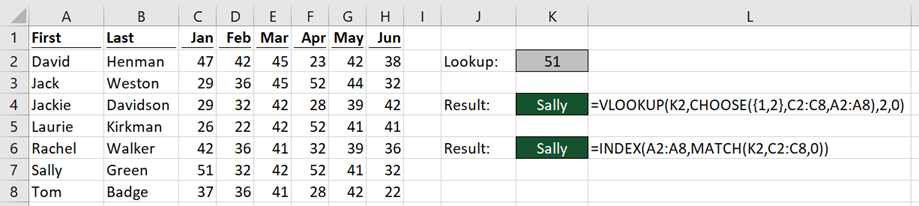
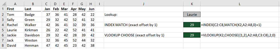
The screenshot above shows how the VLOOKUP CHOOSE combination compares to the INDEX MATCH combination.
Using VLOOKUP it would normally be impossible to lookup a person’s name for a specific value, as the lookup_value is not in the left-most column. However, the CHOOSE function allows us to create a temporary table with the columns in any order we wish. The formula in Cell K4 is:
=VLOOKUP(K2,CHOOSE({1,2},C2:C8,A2:A8),2,0)
The order of the ranges within the CHOOSE function is important, the lookup column (Cells C2:C8) is first, followed by the column to return the result (Cells A2:A8). By using an array of {1,2} as the index_num, it creates a temporary lookup_array with the columns in the specified order.
As shown in the example above, VLOOKUP is looking up to the left, the very thing which it is claimed it cannot do.
VLOOKUP can cope when with deleting columns
The ranges used within the CHOOSE function are not based on their position on the worksheet, but based on the order in the temporary lookup_array. When used in this way it is possible to delete columns without causing the calculation to return an incorrect result.
The calculation before deleting columns
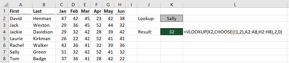
The screenshot above shows the formula result before deleting columns.
The calculation after deleting columns
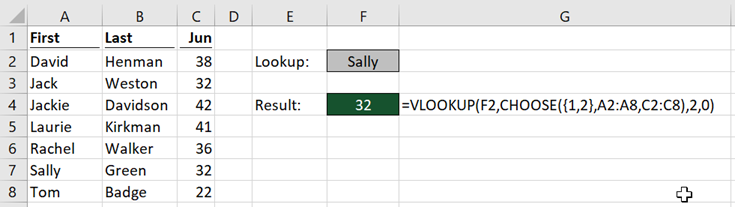
The screenshot above shows the formula after deleting columns (no other changes). By using the CHOOSE function within VLOOKUP, the calculation is correct before and after deleting a column.
VLOOUP is again achieving something else which it is claimed it cannot do.
However …
I have demonstrated that VLOOKUP, when given the right teammate can achieve the same results as INDEX MATCH for basic lookup calculations.
However… this does not make it the better option; INDEX MATCH is the superior combination. It is claimed that INDEX MATCH is harder to understand, if that’s true then users will undoubtedly struggle with VLOOKUP CHOOSE.
The real reason INDEX MATCH is better
The real benefits of INDEX MATCH are much further reaching than as an alternative for VLOOKUP. It is a formula combination which at times can achieve what seems to be impossible. Let me show you…
Can be significantly faster
In the past, I have performed speed tests between INDEX MATCH and VLOOKUP. There is very little difference between them. But nobody ever said you had to use INDEX and MATCH together within the same cell.
The slowest part of any lookup formula is searching to find the matching value. MATCH and VLOOKUP both perform this search activity. INDEX, in comparison, retrieves a value from a range of cells, and is exceptionally fast.
Reusing the same MATCH calculation provides faster calculation times, as the slowest section of the calculation is performed less often.
Look at the screenshot below. Notice how the formulas in Cells L4 and M4 both reference the MATCH function result in Cell K4. The equivalent VLOOKUP calculations are in Cells L7 and M7.
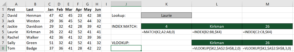
The slower MATCH calculation is only performed once, whilst the fast INDEX function is performed twice.
As VLOOKUP is a single function, it must re-perform the search each time the function is used. This makes VLOOKUP much slower for returning multiple columns from the same table.
Lookup offset
If we want to find a value which is visually above or below the lookup value, which functions could we use? For INDEX MATCH this is no problem, just add or minus an offset number to the result of the MATCH function.
The formula in Cell K4 is:
=INDEX(C2:C8,MATCH(K2,A2:A8,0)+1)
Notice that 1 has been added to the MATCH result, INDEX will return the result one cell below. Use minus 1 to return the cell above.
Can we achieve the same result with VLOOKUP CHOOSE? Yes, if we misalign the two ranges within the CHOOSE function.
The formula in Cell K6 is:
=VLOOKUP(K2,CHOOSE({1,2},A2:A8,C3:C8),2,0)
Notice how the first range (Cells A2 – A8) starts at row 2, whilst the second range (Cells C3-C8) begins at row 3. Whilst this is possible, it’s not a great solution.
INDEX MATCH can perform 5 lookup types
The last argument of VLOOKUP and MATCH indicate the type of search to be performed.
Exact Match
VLOOKUP uses 0 or FALSE as the last argument to perform an Exact match.
MATCH uses 0 as the last argument to perform an Exact match.
Examples of both of these are shown in the screenshot below:
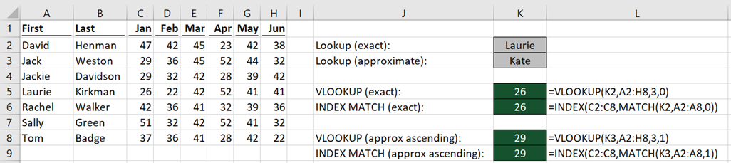
The formula in Cell K5 is:
=VLOOKUP(K2,A2:H8,3,0)
The formula in Cell K6 is:
=INDEX(C2:C8,MATCH(K2,A2:A8,0))
If the item being searched is not in the list, both formulas will return a #N/A.
Approximate Match – Sorted Ascending List
VLOOKUP uses 1 or TRUE as the last argument to perform an Approximate Match on a sorted ascending list.
MATCH uses 1 as the last argument to perform an Approximate Match on a sorted ascending list.
If the item is not in the list, both functions will return the value which is before the searched value.
In the example (see above) Kate is searched for with an approximate match, but as Kate is not in the Cells A2-A8, the result returned is for Laurie, which is the value before it.
The formula in Cell K8 is:
=VLOOKUP(K3,A2:H8,3,1)
The formula in Cell K9 is:
=INDEX(C2:C8,MATCH(K3,A2:A8,1))
Approximate Match – Sorted Descending List
VLOOKUP does not have an option to calculate based on descending order. You would need helper columns or data re-shaping.
MATCH uses -1 as the last argument to perform an Approximate Match on a sorted descending list.
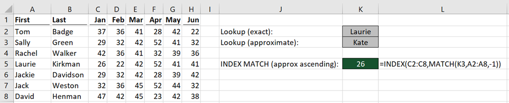
The formula in Cell K5 is:
=INDEX(C2:C8,MATCH(K3,A2:A8,-1))
If the item is not in the list MATCH will return the value which is before the searched value.
Additional Search Types
By combining the lookup offset concept introduced above with the ascending or descending variants, additional search types are created. Normally ascending lists would return the value before, but add one and it will always return the value after . Equally, descending lists can be expanded by using the same offset concept.
With the three match types and the additional two from lookup offset, that makes five in all. This compares with VLOOKUP, which only has two.
INDEX MATCH works over a horizontal range
INDEX MATCH, when used with one-dimensional data, does not care whether the data is arranged vertically or horizontally. Whilst VLOOKUP, by definition, only works with vertically arranged data.
Ah… but what about HLOOKUP? I hear you say. Yes, fair point, but it is a different function, so having to remember which function to use depending on the orientation of the data isn’t ideal.
A reader, David Newell, pointed out to me that it is possible to use the HLOOKUP/CHOOSE combination to lookup a value above. The array is separated by a semicolon, rather than a comma. Here is an example of how the HLOOKUP/CHOOSE combination would be formed.
=HLOOKUP("Tom",CHOOSE({1;2},A2:H2,A1:H1),2,0)
Whilst the HLOOKUP/CHOOSE combination is an option, you’ll rarely, if ever see it used.
INDEX MATCH can lookup an entire row or column
VLOOKUP can only return a single value. But INDEX MATCH can return an entire column of value. The example below shows it is possible to lookup the total value across all the columns without the need for a total column.
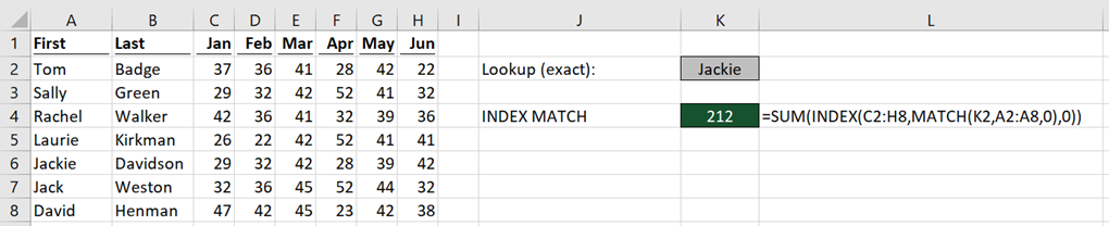
Cell K4 in the screenshot above shows the total of January to June for Jackie. The formula in Cell K4 is:
=SUM(INDEX(C2:H8,MATCH(K2,A2:A8,0),0))
The two things I would like you to notice are:
- The INDEX range is referencing all the Cells C2 – H8, rather than a single row or column
- An additional “,0” (or just an additional “,” (comma)) tells INDEX to return the entire row of data.
All the values (29, 32, 42, 38, 39 and 42) from row 6 are returned. It is not apparent that this has happened as Excel will only display the first result. By wrapping INDEX MATCH within the SUM function, it will add all the values together.
=SUM(INDEX(C2:H8,MATCH(K2,A2:A8,0),0))
The result of the formula is 212, which proves the entire row of data has been returned, rather than a single cell.
INDEX MATCH can create a dynamic range
We saw in the last example that INDEX MATCH could lookup an entire row or column. But what if we only want to look up a specific range within the rows and columns. In the screenshot below two INDEX MATCH formulas are separated by a colon ( : ). This creates a range, which starts at the cell of the first result and finishes at the cell of the second result.
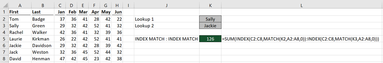
The formula in Cell K5 is:
=SUM(INDEX(C2:C8,MATCH(K2,A2:A8,0)):INDEX(C2:C8,MATCH(K3,A2:A8,0)))
The result of the first INDEX MATCH is Cell C3, the result of the second INDEX MATCH is C6. When separated by a colon this creates the range C3:C6.
The SUM function has been added to show that a range is returned, as values 29, 42, 26 and 29 (from Cells C3-C6) total the result displayed of 126.
Can perform array formulas without Ctrl + Shift + Enter
When creating array formulas, such as matching multiple criteria, both INDEX MATCH and VLOOKUP CHOOSE can achieve the result. The screenshot below shows the result when combining the first and last names as the lookup_value.
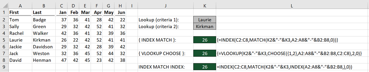
The formula in Cell K5 is:
{=INDEX(C2:C8,MATCH(K2&"-"&K3,A2:A8&"-"&B2:B8,0))}
The formula in Cell K7 is:
{=VLOOKUP(K2&"-"&K3,CHOOSE({1,2},A2:A8&"-"&B2:B8,C2:C8),2,0)}
Both of these are array formulas and will only calculate correctly if Ctrl + Shift + Enter is pressed when entering the formula into the cell or formula bar. Do not add the curly braces ( { } ), Excel will add those by itself.
But here is the magic. By adding another INDEX inside the MATCH, it is possible to avoid the need for Ctrl + Shift + Enter.
=INDEX(C2:C8,MATCH(K2&"-"&K3,INDEX(A2:A8&"-"&B2:B8,0),0))
As we’ve seen previously, INDEX can return multiple values at the same time. In this example, it is combining each cell combination together. “,0” has been used as before to tell INDEX to return all the values. INDEX will convert the array section of the formula into multiple values which can be processed by the MATCH function.
The formula calculates the correct result without Ctrl + Shift + Enter.
Technically, the INDEX function can be added to the VLOOKUP/CHOOSE combination to avoid the array formula. But that’s adding in a third function, which is just adding more complication.
INDEX MATCH follows the logic of Excel Tables
Excel Tables use structured references, where a data table can be referenced using the column headers. Whilst it is possible to use VLOOKUP to retrieve a value from a specific column, it takes away the benefits gained from using a Table.
Normally, a column number within VLOOKUP is just a number, which happens to retrieve the value from the correct column. INDEX MATCH can use structured references in all the ranges, making it is much easier to understand the calculated result.
The one thing VLOOKUP CHOOSE does better
There are certain data handling rules, which if followed make a spreadsheet easy to manage. But guess what, most Excel users have no idea about this, so we can find data structured in some “interesting” ways. The reference form of INDEX can tackle some of this by performing a lookup on multiple tables.
Look at the screenshot below. How can you write a simple formula which will lookup into the correct month of data?
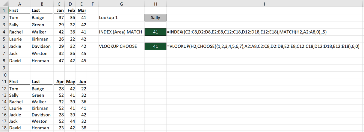
The formula in Cell H4 is:
=INDEX((C2:C8,D2:D8,E2:E8,C12:C18,D12:D18,E12:E18),MATCH(H2,A2:A8,0),,5)
There are multiple ranges (all contained within the parentheses) of the first argument. Each range contains the cell references for each month. The last argument, which is area_num, determines which range to retrieve the result from. In the example above 5 is used, so the 5th area D12:D18 will be used to return the result. Change the area_num to 2 and the 2nd range (Cells D2 – D8) will be used.
Note: This feature only works where the ranges within the first argument of the INDEX function are all contained on a single sheet.
The VLOOKUP CHOOSE formula in Cell H6 is:
=VLOOKUP(H2,CHOOSE({1,2,3,4,5,6,7},A2:A8,C2:C8,D2:D8,E2:E8,C12:C18,D12:D18,E12:E18),6,0)
To lookup into the 5th area using VLOOKUP CHOOSE it is necessary to reference the 6th area, as the lookup column is the 1st reference.
In this scenario, the formulas produce the same result. However VLOOKUP CHOOSE can refer to tables on different sheets, which in some circumstances will make it the better choice, but hopefully, that is very rare.
Other advanced uses for INDEX / MATCH
Another great use for INDEX / MATCH is to use it as a picture lookup formula.
Conclusion
After all the things I have shown you, I hope you agree that INDEX MATCHit is not just a replacement for VLOOKUP.
VLOOKUP by itself is just not comparable to INDEX MATCH. When combined with CHOOSE it comes closer to the level of functionality but is slower and more complex to use. INDEX MATCH is an amazing formula combination which can perform Excel magic.
Do I still use VLOOKUP? Of course I do. For simple data tables it is still a great solution. As complexity increases, INDEX MATCH becomes the better option.
Discover how you can automate your work with our Excel courses and tools.
The Excel Academy

Make working late a thing of the past.
The Excel Academy is Excel training for professionals who want to save time.
Mark, this is truly off the grid! Next thing we know, you’ll be designing printed circuit boards in Excel!
I’m one of those who find it a challenge to keep the Index Match parameter spaghetti straight. After really digging into your article, though, I’m convinced that I can follow the logic well enough to create some cool lookup formulas. (After all, I can put the base formulas into VBA and generate them dynamically!)
Thanks for the informative, in-depth look into Index Match.
This is going into my Evernote for reference!
Cheers,
Mitch
Hi Mitch,
Thank you – I appreciate your comments.
If I knew anything about printed circuit boards, then I certainly would try to use Excel for that 🙂
Hi Mark
by far the best post on VLOOKUP, INDEX & MATCH that I have seen up to now (appart from my own of course 🙂 )
Another thought on why it may be that in general people find VLOOKUP easier: Because they usually learn that one first. Therefore by the time they get to the INDEX / MATCH combination they are already lots ahead with VLOOKUP practice.
have fun and thanks for your post – Bruno
Hi Bruno,
Thank you, that is very kind of you to say.
In regard to your point about learning VLOOKUP first, I agree completely. I have a similar thought about array formulas. If arrays were taught on simple formulas I’m sure people would find it easier to pickup. But I don’t know anybody who has tried it, so it’s just a thought.
Great post. Another place where INDEX/MATCH does better is when you don’t know what range your matching on. You can either use a nested index/match:index/match to find the range or if you wanted to used a volatile formula, got that from a previous post :), you could use an OFFSET. Basically, decoupling the match and return range provides insane flexibility. Shun the non-believers of INDEX/MATCH!!
Hi Will,
That’s a good idea. I don’t think I’ve ever tried an INDEX/MATCH dynamic range inside a MATCH, but it should definitely work, I use the same approach with slow formulas, it narrows down the range before applying the slower functions.
I would suggest that you haven’t really debinked “VLOOKUP can only lookup to the right”. It takes an enormously heroic effort to lookup to the left, whereas with Index-Match, looking up in any direction is easier and more intuitive.
Hi Jon,
I have used the word “debunked” quite liberally. I would agree, INDEX MATCH a significantly better option, maybe I should make that clearer in the post itself.
Great article.
I think you have undervalued the technique you used in the dynamic range example. The INDEX functions are returning references rather than values and this is a powerful technique that VLOOKUP does not have. VLOOKUP cannot return a reference to a cell – INDEX can.
Also it is worth noting that you can use MATCH with VLOOKUP to handle the column lookup when columns are inserted /deleted.
Thanks Neale – both are good points.
Name Color Name Color
Mike ? Tom
Richard ? Orange
Tom ? Richard
Blue
Mike
Green
I’d like to write a formula that would return Green, Blue and Orange in teh second column next to the names in the first column. I tried INDEX MATCH and failed.
Any suggestions?
Sorry, but the format of your sample data hasn’t come out that well. So I’m not quite sure what outcome you’re looking for.
Another fine article made obsolete by XLOOKUP!
The good news is that old habits die hard, so there is probably a few more months of life in this post before it gets retired 🙂