
I love using the double VLOOKUP trick to get some lighting fast calculation times in Excel. The drawback is that the list being looked up has to be sorted to prevent errors. If a list were not sorted, it would be great to see a warning. Then the user can take action to sort the list before continuing.
This post will consider three formula methods to find out if a list is sorted.
- Helper column
- Array formula
- Array formula for tables
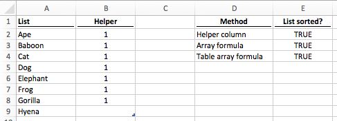
If the list is sorted the formulas show True
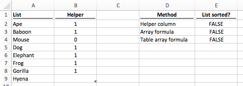
If the list is unsorted, the formulas show False
Helper column approach to check if a list is sorted
Of the three options, the helper column approach is probably the worst, but the easiest to understand. This method uses a Helper column to find out if each value is lower than the value in the cell below it. If all the results are True, then the list is sorted.
The formula in Cell B2 is:
=(A2<=A3)*1
Where A2 is less than A3 the result will be True, otherwise it will be False. This is then multiplied by 1 to return a value of 1 or zero. The formula is copied down to the last-but-one cell of the list.
The formula in Cell E2 is:
=PRODUCT(B2:B8)=1
The PRODUCT function multiplies the results of the Helper column together. If all the results in the Helper column are 1 then the result of the PRODUCT function is 1. However, if any of the results in the Helper column is 0, the result of the PRODUCT function will also be 0.
Array formula to check if a list is sorted
Normally, array formulas are a bit tricky, but in this circumstance, it is easy enough to follow.
The formula in Cell E3 is:
{=AND(A2:A8<=A3:A9)}
As this is an array formula, do not type the curly braces ( { } ) at the start or end of the formula. But do press Ctrl + Shift + Enter when entering the formula.
The formula works by moving down each range and comparing the cells as pairs. Is A2 <= A3, then is A3 <= A4, then A4<=A5 and so on, until the bottom of the range of cells. Wrapping this within the AND function will result in True only if all the cell combinations are True. If any are False the final result will be False.
Array formula for tables to check if a list is sorted
Combining the array formula with an Excel Table starts to get a bit tricky. The List column (Column A in our example) is part of a table called Table1. On the screenshot, at the start, it may not look like an Excel Table, as I have removed the formatting.
The formula in Cell E4 is:
{=AND(INDEX(Table1[List],1):INDEX(Table1[List],ROWS(Table1[List])-1)
<=INDEX(Table1[List],2):INDEX(Table1[List],ROWS(Table1[List])))}
The formula shown is on two lines here because the web-page is not wide enough, but it can be shown on a single line in the Formula Bar of Excel. Again, this is an array formula, so don’t type curly braces, but do press Ctrl + Shift + Enter to enter the formula.
That formula looks pretty complex, right? But it is actually the same as the normal array formula shown above, but adapted to work with Excel Tables. Let’s break down the formula
INDEX(Table1[List],1)
The first index function returns the cell address for the first cell in the List column of Table 1.
INDEX(Table1[List],ROWS(Table1[List])-1)
The second index function uses the ROWS function to count the number of rows in the List column of Table1, then it reduces the value by 1. In our example, there are 8 rows in the List, column so the ROWS function will return 7 (8 rows minus 1). The index function returns the cell address for the 7th cell in the List column of Table 1. So far, our formula will just be A2:A8 (A2 is the first row in the List column, A8 is the 7th row in the List column).
INDEX(Table1[List],2):INDEX(Table1[List],ROWS(Table1[List]))
The next two INDEX functions follow a similar method. The first INDEX returning the 2nd item in the list and the second INDEX returning the last item in the list, so the cell ranges are A3:A9.
The remainder of the formula is the same as the basic array formula above. Even though it appears more complex it achieves exactly the same result. The Excel Table will expand or retract based on the amount of data. This formula will also expand or retract in the same way.
Conclusion
Using any of the methods above it is possible to create a check to ensure a list is sorted. This is especially useful when using a sorted list for a VLOOKUP or MATCH function
Discover how you can automate your work with our Excel courses and tools.
The Excel Academy

Make working late a thing of the past.
The Excel Academy is Excel training for professionals who want to save time.
Do you happen to know of a way to make the array method work when there are any number of blanks in the column? It seems like ideally you’d somehow create temporary helper columns that removed the blanks somehow, and then compare the list itself to the list shifted down one row? But I can’t make that work. Thanks!
Hi Micron,
How about this array formula.
{=AND(IF(A2:A9=””,A1:A8,A2:A9)<=IF(A3:A10="",A2:A9,A3:A10))} The IF within the array makes any blank equal to the cell above. However, if there are multiple rows of blanks one after the other it will not work. Not a perfect solution, but would this work for your situation?
I have a very large set of data (250K rows) that I want to know if I’ve already sorted or not. I was planning on using the helper column approach but I did a quick google search to see if there was anything built-in to Excel to do it even easier and found your column.
My comment is: Instead of creating a PRODUCT formula in a cell, I was just going to turn on filtering, and check for any FALSE entries. Easier to remember the next time I want to do this again.
That is a reasonable option, provided you definitely remember to do it each time the data is updated.
Very cool way to analyze cell to cell! Thanks for the explanation.
In my case, it does not work unless I copy the column, and then paste special back in the same column as Values. I have to do this every single time I make a change and want the array formula to give me a correct answer.
Thanks again for the very nice tutorial.
David
Hi David – I’ve not been able to re-create your issue. Are you about to share some more information about your situatinos.