How to create a PivotTable from multiple Tables (easy way)

When most people use PivotTables, they copy the source data into a worksheet, then carry out lots of VLOOKUPs to get the categorization columns into the data set. After that, the data is ready, we can create a PivotTable, and the analysis can start. But we don’t need to do all those VLOOKUPs anymore. Instead, we can build a PivotTable from multiple tables. By creating relationships between tables, we can combine multiple tables which automatically creates the lookups for us.

The ability to create relationships has been natively available in Excel since 2013, yet most users don’t even know this feature exists.

We don’t need to copy and paste data into a worksheet either as we can now use Power Query to import the data directly. Check out my Power Query series to understand how to do this. But, for this post, we are focusing on creating relationships and how to combine two PivotTables.

Table of Contents

• The scenario
• Create tables
• Creating relationships
• Create the PivotTable
• Refresh a PivotTable from Multiple Tables
• Auto relationship detection
• Duplicate values in lookup tables
• Power Pivot
• Conclusion

Watch the video

Watch the video on YouTube.

The scenario

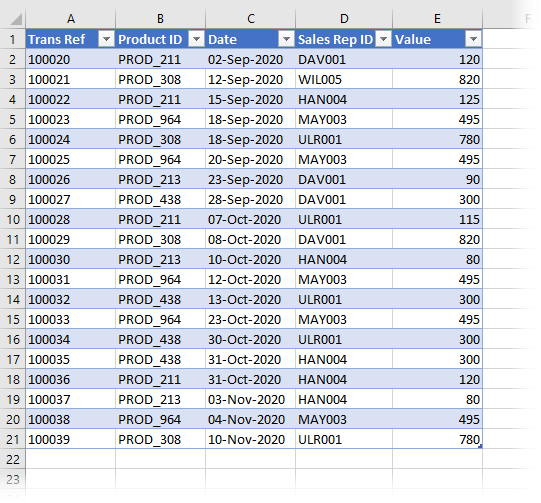
In our example file, we have three sections of data:

• Sales data
• Sales rep data
• Product data

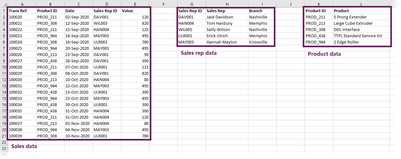
These data sets could be on separate worksheets, but for ease of demonstration, they are included on one.

The sales data contains the transaction information, which is often referred to as a fact table. The sales rep data and product data include the categorization to analyze the transactions; these are often referred to as lookup tables.

Our goal is to create a PivotTable showing product sales by branch. This requires information from all three data tables:

• Product is in the Product data table
• Branch is in the Sales rep data table
• Value is in the Sales data table

To achieve this, we will create relationships to combine PivotTables. We will not use a single formula!

Create tables

First, we need to turn our data into Excel tables. This puts our data into a container so Excel knows it’s in a structured format that can be used to create relationships.

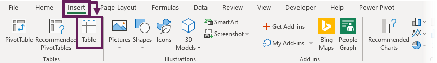
Select any cell within the first block of data and click Insert > Table (or press Ctrl + T).

The Create Table dialog box opens. Check the range includes all the data, and ensure my data has headers is ticked. Then click OK

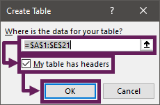
The data changes to a striped format. This is a visual indicator that an Excel table has been created.

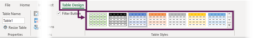
TOP TIP: You don’t need to stick with that format. Click any cell in the table, then click Table Design and choose another format from those available.

Next, we need to give our Table a meaningful name. With any cell in the table selected, click Table Design and enter a new name into the Table Name box. I’ve chosen SalesData (spaces and most special characters are not permitted within table names).

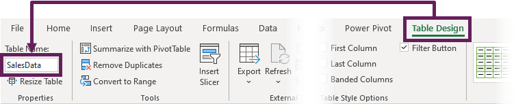
Repeat the steps above for the other datasets to create tables called SalesRepData and ProductData.

Creating relationships

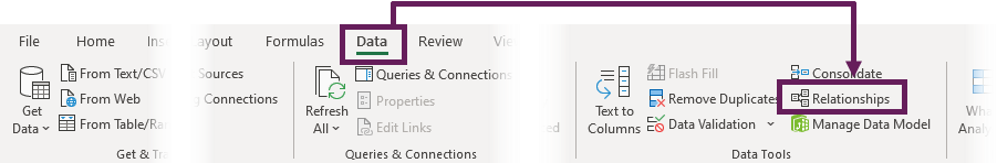
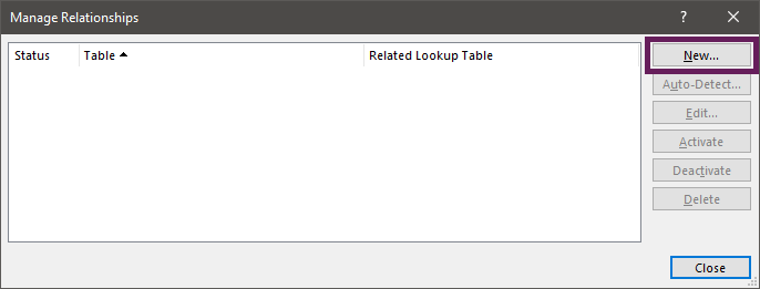
With our three tables created, it’s now time to start creating the relationships. Click Data > Relationships.

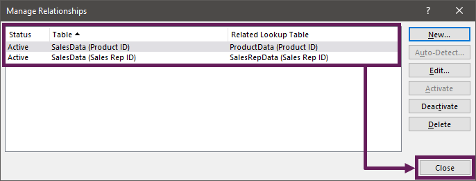
The Manage Relationships dialog box opens. Click New.

The Create Relationship dialog box opens. This is where we define the relationships that exist.

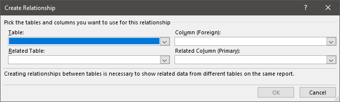
I don’t think the descriptions in this dialog box are particularly clear, so I’ll try to give you a bit of a steer.

• Table: This is the table containing the transactional values that we want to analyze (the fact table).
• Column (Foreign): This is the name of the column from the transactional values table which we want to lookup from. If you’re in the VLOOKUP mindset, then this would be the column containing the lookup_value argument. The word Foreign is database terminology to indicate that this column can have duplicate values.
• Related table: This is the table containing the categories we want to analyze the transactional data by (the lookup table).
• Related Column (Primary): This is the column we want to pair with the Column (Foreign) we selected above. If this were a VLOOKUP, it would be the first column in the table_array argument. The word Primary is database terminology again; it tells us the column must contain unique values.

The columns do not need to share a common header name for this technique to work. However, it can be helpful to remember how the tables are related.

In our example, we use the following:

• Table: SalesData
• Column (Foreign): Sales Rep ID
• Related Table: SalesRepData
• Related Column (Primary): Sales Rep ID

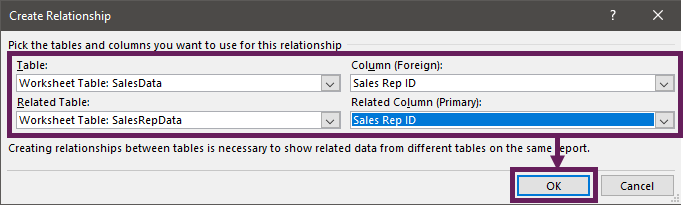
Click OK to create the relationship.

That’s it, simple right! We have just combined two tables without any formulas.

Next, let’s create the relationship between the SalesData and ProductData tables using the same process as above.

• Table: SalesData
• Column (Foreign): Product ID
• Related Table: ProductData
• Related Column (Primary): Product ID

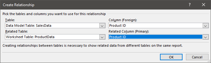
Once all the relationships are created, click Close.

Create the PivotTable

Everything is in place, so we are now ready to create the PivotTable.

Click Insert > PivotTable from the ribbon.

The Create PivotTable window opens. The most important thing is the Use this workbook’s Data Model option is selected.

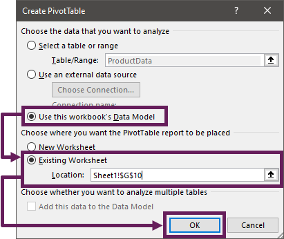
Select a location to create the PivotTable. For this example, we will make the PivotTable on the same worksheet as the data. I’ve selected the Existing Worksheet in cell Sheet1, Cell G10, but you can put your Pivot Table wherever you like.

Click OK to close the Create PivotTable dialog box.

The PivotTable is created. Notice that the PivotTable Fields window includes all three tables. We can now start dragging fields from each table to form a single view.

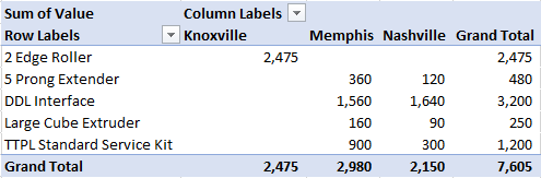
As I said earlier, the goal is to show product sales by branch. To achieve this, put the fields into the following sections:

• Columns: SalesRepData > Branch
• Rows: ProductData > Product
• Values: SalesData > Sum of Value

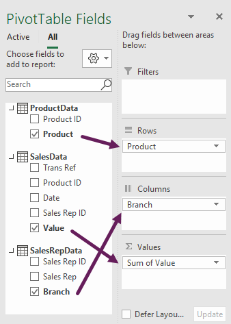
If you don’t see all the tables in the PivotTable Fields view, then change the selection from Active to All.

This creates the following PivotTable:

There you have it. We’ve created a PivotTable from multiple tables without any formulas 😁.

Refresh a PivotTable from Multiple Tables

Whether the data comes from a single table or multiple tables, the refresh process is the same. Click Data > Refresh All in the ribbon.

However, there are advanced options we can use, which are not available for standard PivotTables:

• Click Data > Queries & Connections to view all the connections in the workbook.
• Right-click on one item in the Connections list and select Properties from the menu.
• The Connection Properties dialog box opens.

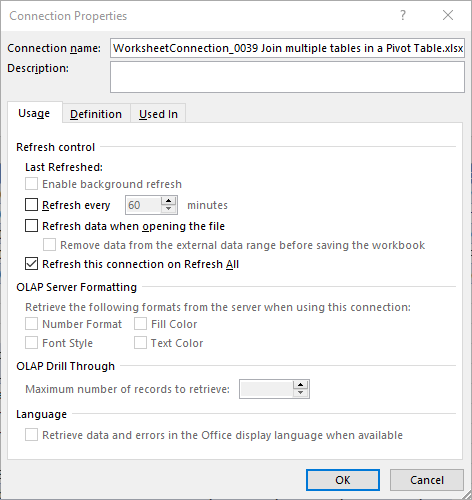
While many options in here are greyed out, there are options to:

• Refresh every x minutes
• Refresh data when opening the file
• Refresh this connection on Refresh All

These are especially useful if working with external data connections.

Auto relationship detection

When working with relationships, you may find opportunities to Auto-Detect relationships. For example, Excel may display the following message.

“Relationships between tables may be needed“

DO NOT click the Auto-Detect button. If you do, Excel will try to use its own logic to build relationships. In a simple scenario, it will work, but Excel often gets it wrong. If necessary, go back to the Relationships dialog box and check that everything is set up and calculating correctly. If it is working correctly, then ignore the warning message.

Duplicate values in lookup tables

If there are duplicate values in our lookup tables (or related tables as they are called in the Relationships window), this causes an error and the relationships won’t work.

When we use lookup functions such as VLOOKUP, XLOOKUP, or INDEX/MATCH, Excel always returns the first item, even if it’s not the answer we want. But when we use relationships, if there is more than one matching value, Excel doesn’t know which item to use. This causes the error. Therefore, to ensure the integrity of our data, we must have unique values in our lookup tables.

Creating a relationship with duplicate values

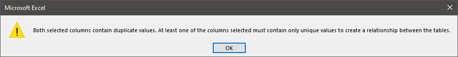
When creating the relationship, if there are duplicate values in our lookup table, we will get the following error:

“Both selected columns contain duplicate values. At least one of the columns selected must contain only unique values to create a relationship between the tables.“

We must go back and fix our source table before we create the relationship.

Adding duplicate values into a table?

If we accidentally add duplicate values to our lookup tables, we get an error when refreshing the PivotTable.

We couldn’t refresh the connection ‘__________’. Here’s the error message we got:
Column ‘__________’ in Table ‘__________’ contains a duplicate value ‘__________’ and this is not allowed for column on the one side of a many-tone relationship of for columns that are used as the primary key of a table.

We must go back and fix the data in the lookup table and then the refresh again.

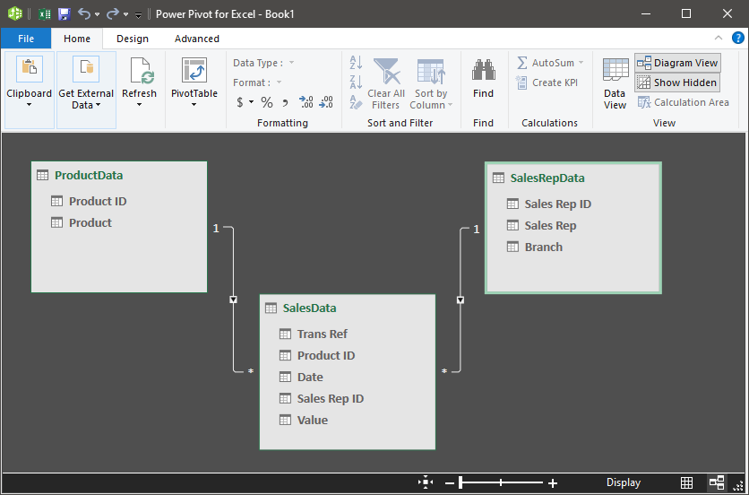
Power Pivot

You probably didn’t realize, but you’ve just used the Power Pivot engine in Excel. We’ve not opened or enabled the Power Pivot add-in; all we’ve used is the standard Excel interface. However, if we were to open the Power Pivot tool, we would see that our data and relationships exist.

Conclusion

In this post, we’ve created a PivotTable from multiple tables without formulas, something which was not possible before Excel 2013.

If you understand how these relationships work, maybe it’s time to investigate Power Pivot a bit further. Then you can gain even more automation benefits and create even more advanced reports.

---

What next?

Discover how you can automate your work with our Excel courses and tools.