Create Slopegraphs in Excel

I’m not going to lie to you, the first time I saw a slopegraph, I was completely underwhelmed, I thought “it’s just a line chart with two points, hardly worth getting excited about”.  But the reaction, the first time I used one in a presentation, was unbelievable. People even asked me for my template, so they could create slopegraphs themselves. In this post, I want to show you how to create slopegraphs in Excel.

Table of Contents

• What are slopegraphs?
• Fixed format slopegraph
• The data
• Create the chart
• Formatting the chart
• Create automatically with vba macro
• Dynamic format slopegraph
• The data
• Create the chart
• Create automatically with vba macro
• Conclusion

Watch the video

Watch the video on YouTube.

What are slopegraphs?

Slopegraphs were first introduced by Edward Tufte in 1983.  But, I believe, it is only in recent years, with the increase in data visualization that this chart has been brought to the attention of the masses.

They work so well because our brains are good at comparing slopes/angles.  They are useful for comparing two points that are equivalent to each other but separated by time or a specific event.  Good uses would be product margin between months, or company profits across years.

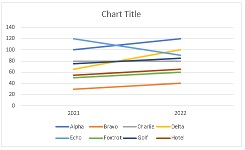
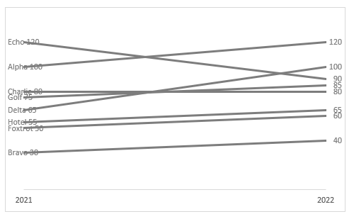
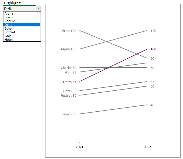
Look at the chart below – what does it tell you?

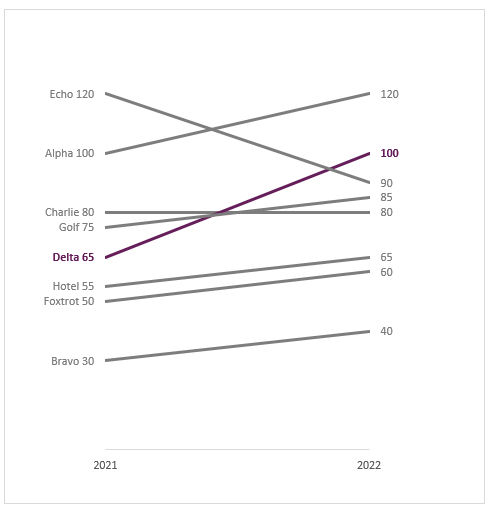
With just a brief glance, the slopegraph shows that Delta has significantly increased. Even without highlighting, we can see that Alpha has increased and Echo has decreased.  Simple, no brain power needed. The slopes/angles give us an easy way to understand the story.

Fixed format slopegraph

Let’s start with a fixed format slopegraph. This is a static visualization, so we need to update the colors manually if we want to highlight different items.

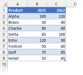
The data

The data we will be using in this example is as follows:

Create the chart

The chart is based on a standard line chart.

1. Select a cell inside the Table.
2. From the ribbon, click Insert > Charts > Line Chart
   
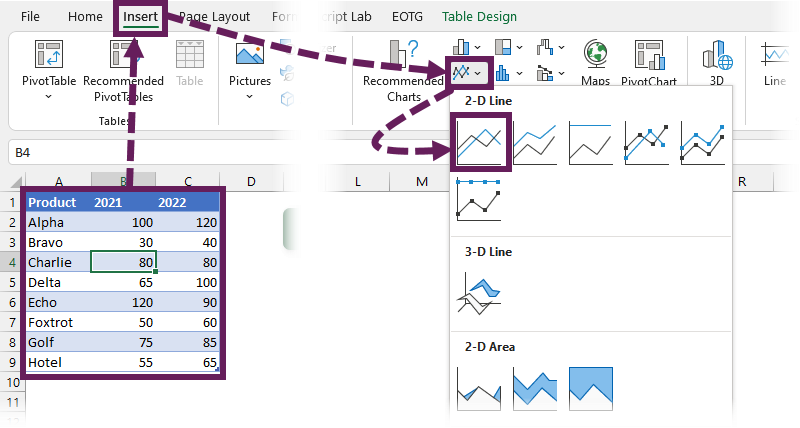
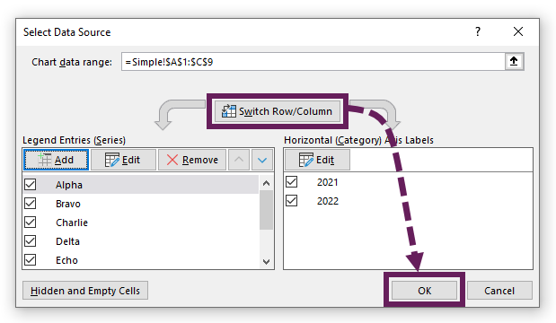
3. The standard line chart appears. Right-click on the chart area, from the menu, click Select Data….
   
   
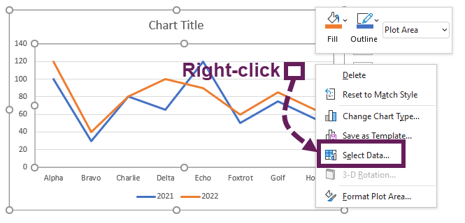
4. Within the Select Data Source dialog box, there are two main boxes (The left box contains years; the right box contains the products).  We need to switch these over.  Click the Switch Row/Column button, then clickOK
   

Now we are starting to get somewhere.  We’ve not even formatted this chart and it’s already starting to tell us some key stories.

Formatting the chart

Now, let’s start formatting the chart.  The quick and simple formatting is:

• Delete the legend (the box containing the colored key at the bottom).
• Change, format or delete the title (in the example file, I have deleted it)
• Delete the major gridlines
• Delete the left axis (radical, I know).
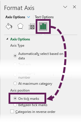
• Right-click on the bottom axis and select Format Axis…</strong from the menu.
  
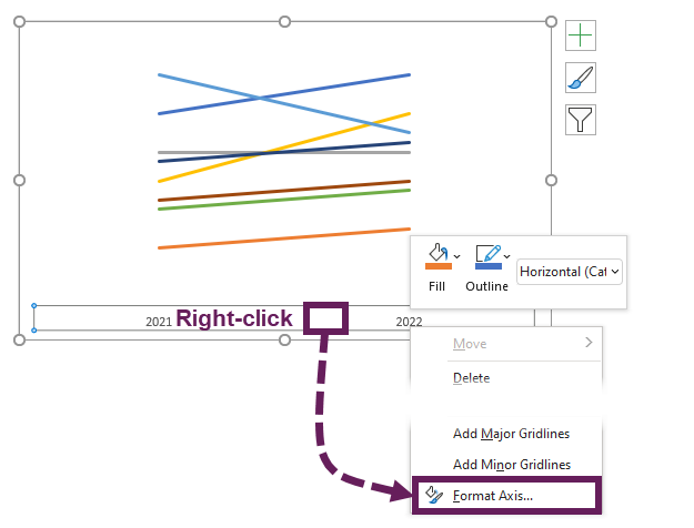
  From the Format Axis panel select On tick marks.
  

The next bit of formatting is quite time-consuming as we have to apply it line by line; it would be great to do it all in one go, but unfortunately, Excel doesn’t want to work that way.

• Right-click on a line, from the menu click Format Data Series… 
  
  
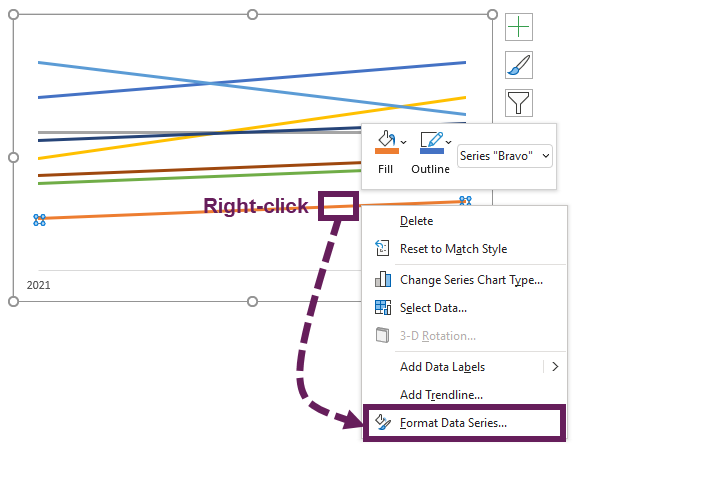
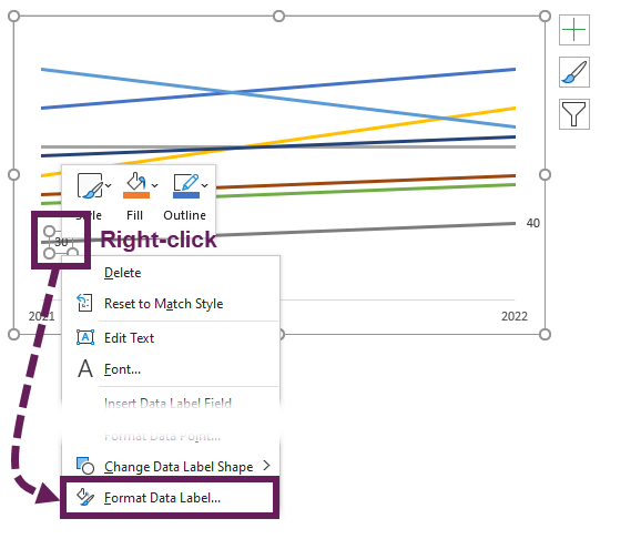
• From the Format Data Series panel click on the Paint Can > Line option> Solid line, then select a color.  I recommend using a mid-grey for anything which isn’t worth highlighting.
  
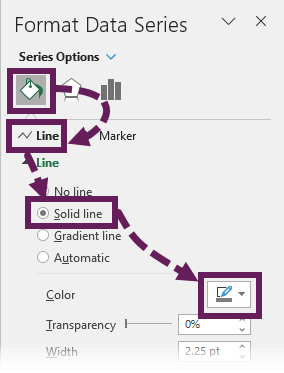
• Now, let’s get the data labels sorted out.  Right-click on the line and select Add Data Labels from the menu.
  
• Set the label text color to be the as the line (i.e. the same grey color).
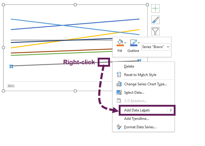
• Click twice on the data label on the left (it should now have empty white dots surrounding it), then right-click and select Format Data Label…
  
  
• From the Format Data Label panel selects the following:
  • Series Name – selected
  • Value – selected
  • Separator – (space)
  • Label Position – Left

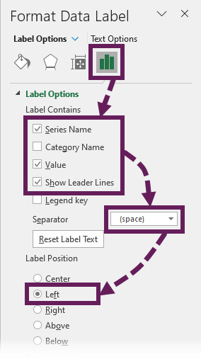
• Format the data label on the right, in a similar way, but do not include the Series Name; we only need the Value.

Repeat the formatting steps above for each line – a bit of a pain, I know.

The chart should now look like this:

Now, it’s time for the final edits:

• Change the width of the plot area
• Change the size of the chart to be taller rather than wider.

Finally, Change the color for any items you wish to highlight, and make the data labels the same color as the line.

Looks pretty good, right?

It took quite a bit of formatting, but we got there in the end.

Create automatically with vba macro

All that formatting takes quite a while. So, I wrote the following macro to handle it for us. Add the code to a standard code module.

For the macro to work, the data must be stored in an Excel Table with the columns in the same order as the example above. The column headings can be different, but the column order must be the same.

To adapt the code to your needs, change the highlightCodeColor and highlightRowIndex parameters.

To execute the macro, select a cell inside the Excel Table and run the Macro.

Sub createSimpleSlopegraph()

Dim ws As Worksheet
Dim tbl As ListObject
Dim cht As Chart
Dim srs As Series
Dim i As Long
Dim standardColorCode As Long
Dim highlightColorCode As Long
Dim highlightRowIndex As Long

'Select the colour to use for highlighting
standardColorCode = RGB(125, 125, 125)
highlightColorCode = RGB(102, 30, 91)

'Which row to highlight
highlightRowIndex = 4

'Assign the variables
Set ws = ActiveSheet

'Select the table to build the Slopegraph from
On Error Resume Next
Set tbl = ActiveCell.ListObject
On Error GoTo 0
If tbl Is Nothing Then
    Exit Sub
End If

'Create the chart
Set cht = ws.Shapes.AddChart.Chart

'Delete any defaults already applied
For Each srs In cht.SeriesCollection
    srs.Delete
Next srs

'Delete the legend
cht.Legend.Delete

'Delete chart title
If cht.HasTitle = True Then
    cht.ChartTitle.Delete
End If

'Delete the value Axis
cht.Axes(xlValue).Delete

'Remove the gridlines
cht.Axes(xlValue).MajorGridlines.Delete

'Add a new chart series for each row in Table
For i = 1 To tbl.ListRows.Count

    Set srs = cht.SeriesCollection.NewSeries

    With srs
        .Values = ws.Range(tbl.ListColumns(2).DataBodyRange(i, 1), _
            tbl.ListColumns(3).DataBodyRange(i, 1))
        .XValues = ws.Range(tbl.HeaderRowRange(2), tbl.HeaderRowRange(3))
        .Name = "='" & ws.Name & "'!" & tbl.ListColumns(1). _
            DataBodyRange(i, 1).Address
        .ChartType = xlLine
        .Format.Fill.Visible = msoTrue
        .HasDataLabels = True
        If i = highlightRowIndex Then
            .Format.Line.ForeColor.RGB = highlightColorCode
            .DataLabels.Format.TextFrame2.TextRange.Font.Fill.ForeColor. _
                RGB = highlightColorCode
            .DataLabels.Format.TextFrame2.TextRange.Font.Bold = msoTrue
        Else
            .Format.Line.ForeColor.RGB = standardColorCode
            .DataLabels.Format.TextFrame2.TextRange.Font.Fill.ForeColor. _
                RGB = standardColorCode
        End If
    End With

    With srs.Points(1)
        .DataLabel.Position = xlLabelPositionLeft
        .DataLabel.ShowSeriesName = True
        .DataLabel.ShowValue = True
        .DataLabel.Separator = " "
    End With

    With srs.Points(2)
        .DataLabel.Position = xlLabelPositionRight
        .DataLabel.ShowSeriesName = False
        .DataLabel.ShowValue = True
    End With

Next i

'Set chart to on tick marks
cht.Axes(xlCategory).AxisBetweenCategories = False

'Change width of plot area
cht.PlotArea.Width = cht.ChartArea.Width * 0.6
cht.PlotArea.Left = cht.ChartArea.Width * 0.2

End Sub

Dynamic format slopegraph

If we include slopegraphs on regularly updated reports, or dynamic dashboards, we do not want to manually change colors.  So, let’s create a slopegraph that can dynamically highlight specific lines.

Excel Charts have a useful feature whereby the #N/A value is not rendered on the chart. We make use of this a lot when creating dynamic charts.

The data

We will use the same data as the previous example, but now we have added some duplicate the columns (don’t worry all will become clear).

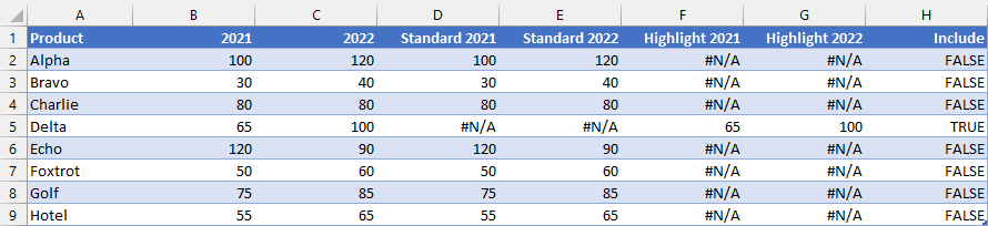
The formulas in the Table are as follows:

Cell H2 (Include column):

=[@Product]=$J$3

Cell J3 contains the name for the line we want to highlight. In the data screenshot above, Delta has been selected, therefore this item shows TRUE in the Include column.

Cell D2 (Standard 2021 column):

=IF(tblDataDynamic[@[Include]:[Include]]=TRUE,NA(),[@2021])

Cell D2 contains logic that if the Include column is TRUE then show #N/A, otherwise display the value from 2021.

Cell E2 (Standard 2022 column):

=IF(tblDataDynamic[@[Include]:[Include]]=TRUE,NA(),[@2022])

Cell E2 contains the same logic as above, but returns the value from 2022.

Cell F2 (Highlight 2021 column):

=IF(tblDataDynamic[@[Include]:[Include]]=TRUE,[@2021],NA())

Cell F2 contains logic that if the Include column is TRUE then return the value from 2021, otherwise return #N/A.

Cell G2 (Highlight 2022 column):

=IF(tblDataDynamic[@[Include]:[Include]]=TRUE,[@2022],NA())

Cell G2 contains the same logic as above, but returns the value from 2022.

Formula Summary

The formulas above ensure that the values exist in either the Standard columns or the Highlight columns, but never both. Have another look at the Table screenshot above.

• Alpha has values in the Standard, but the Highlight columns show #N/A.
• Delta (the selected item) has values in Highlight, but shows #N/A in the Standard columns.

Create the chart

Using the values in the Product, Standard 2021 and Standard 2022 columns create a chart using exactly the same method as the fixed format shown above, keeping all the lines mid-grey.

Now add chart series for each row using the values in the Highlight 2021 and Highlight 2022 columns.

• Right-click on the chart, from the menu, click Select Data…
• In the Select Data Source dialog box, click Add
• Add the series name and series values for that row of the Table, then click OK.

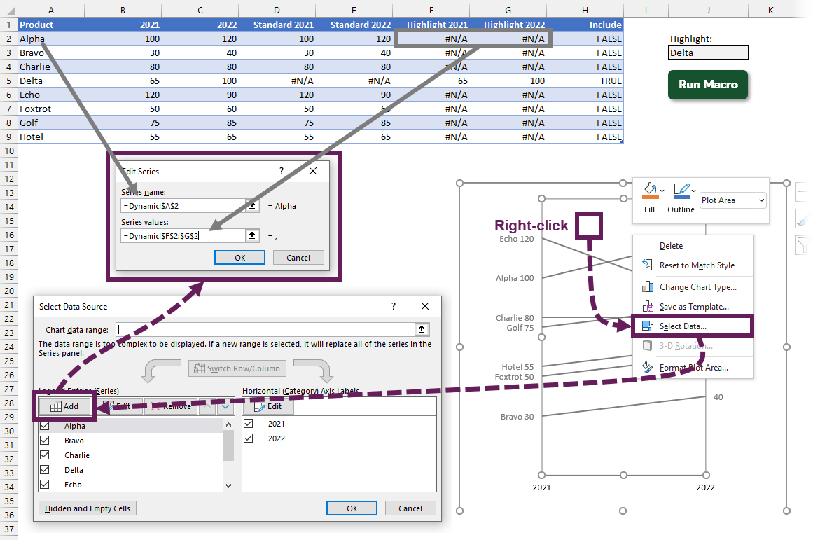
Repeat these actions for every row in the Excel Table.

The slopegraph will now have the original data from the Standard columns, with the values from the Highlight columns placed directly over the top.

Format the new highlight lines in the color you wish to use.

As the #N/A values are not displayed on the chart, you will need to change the value parameters to ensure you have formatted every line correctly.

I’ve connected cell J3 to a data validation list.  After formatting the chart, it will look like this:

If we want to highlight a different line, we can simply select another item from the data validation list.

Create automatically with vba macro

Let’s save ourselves a lot of formatting time, shall we? Once again, we can simply click a cell inside the Table and run the following VBA Macro.

The code should be entered in a standard code module, and the columns must be in the same order as shown in the section directly above.

To adapt the code to your needs, you will need to change the highlightCodeColor.

Sub createDyanamicSlopegraph()

Dim ws As Worksheet
Dim tbl As ListObject
Dim cht As Chart
Dim srs As Series
Dim i As Long
Dim standardColorCode As Long
Dim highlightColorCode As Long

'Select the colour to use for highlighting
standardColorCode = RGB(125, 125, 125)
highlightColorCode = RGB(102, 30, 91)

'Assign the variables
Set ws = ActiveSheet

'Select the table to build the Slopegraph from
On Error Resume Next
Set tbl = ActiveCell.ListObject
On Error GoTo 0
    If tbl Is Nothing Then
    Exit Sub
End If

'Create the chart
Set cht = ws.Shapes.AddChart.Chart

'Delete any defaults already applied
For Each srs In cht.SeriesCollection
    srs.Delete
Next srs

'Delete the legend
cht.Legend.Delete

'Delete chart title
If cht.HasTitle = True Then
    cht.ChartTitle.Delete
End If

'Delete the value Axis
cht.Axes(xlValue).Delete

'Remove the gridlines
cht.Axes(xlValue).MajorGridlines.Delete

'Add a new chart series for each row in Table
For i = 1 To tbl.ListRows.Count

    Set srs = cht.SeriesCollection.NewSeries

        With srs
            .Values = ws.Range(tbl.ListColumns(4).DataBodyRange(i, 1), _
                tbl.ListColumns(5).DataBodyRange(i, 1))
            .XValues = ws.Range(tbl.HeaderRowRange(2), tbl.HeaderRowRange(3))
            .Name = "='" & ws.Name & "'!" & tbl.ListColumns(1). _
                DataBodyRange(i, 1).Address
            .ChartType = xlLine
            .Format.Line.ForeColor.RGB = standardColorCode
            .HasDataLabels = True
            .DataLabels.Format.TextFrame2.TextRange.Font.Fill.ForeColor. _
                RGB = standardColorCode
        End With

    With srs.Points(1)
        .DataLabel.Position = xlLabelPositionLeft
        .DataLabel.ShowSeriesName = True
        .DataLabel.ShowValue = True
        .DataLabel.Separator = " "
    End With

    With srs.Points(2)
        .DataLabel.Position = xlLabelPositionRight
        .DataLabel.ShowSeriesName = False
        .DataLabel.ShowValue = True
    End With

Next i

'Add the highlight series for each row in the Table
For i = 1 To tbl.ListRows.Count

    Set srs = cht.SeriesCollection.NewSeries

    With srs
        .Values = ws.Range(tbl.ListColumns(6).DataBodyRange(i, 1), _
            tbl.ListColumns(7).DataBodyRange(i, 1))
        .XValues = ws.Range(tbl.HeaderRowRange(4), tbl.HeaderRowRange(3))
        .Name = "='" & ws.Name & "'!" & tbl.ListColumns(1). _
            DataBodyRange(i, 1).Address
        .ChartType = xlLine
        .Format.Line.ForeColor.RGB = highlightColorCode
        .HasDataLabels = True
        .DataLabels.Format.TextFrame2.TextRange.Font.Fill.ForeColor. _
            RGB = highlightColorCode
        .DataLabels.Format.TextFrame2.TextRange.Font.Bold = msoTrue
    End With

    With srs.Points(1)
        .DataLabel.Position = xlLabelPositionLeft
        .DataLabel.ShowSeriesName = True
        .DataLabel.ShowValue = True
        .DataLabel.Separator = " "
    End With

    With srs.Points(2)
        .DataLabel.Position = xlLabelPositionRight
        .DataLabel.ShowSeriesName = False
        .DataLabel.ShowValue = True
    End With

Next i

'Set chart to on tick marks
cht.Axes(xlCategory).AxisBetweenCategories = False

'Change width of plot area
cht.PlotArea.Width = cht.ChartArea.Width * 0.6
cht.PlotArea.Left = cht.ChartArea.Width * 0.2

End Sub

Conclusion

As we have seen, slopegraphs are a bit of a pain to set up, but with a macro, we can create them quite quickly. Personally, I think it is worth the effort, as they are beautiful in their storytelling simplicity.

---

What next?

Discover how you can automate your work with our Excel courses and tools.