INDEX MATCH MATCH in Excel (How to do 2-dimension lookup)

In this post, I want to cover one of the most powerful lookup functions available in Excel, INDEX MATCH MATCH. Actually, to call it a function is poor terminology, as it’s three functions used together within a formula. It allows us to return a result based on a lookup from rows and columns at the same time.

If you are familiar with the INDEX MATCH function, this post should not be too much of a stretch for you, as the principles are the same. However, if you’re not familiar with it, don’t worry, I will explain everything.

Table of Contents

• When to use INDEX MATCH MATCH
• Applying the INDEX MATCH MATCH formula
• MATCH
• INDEX
• Nesting MATCH inside INDEX
• Common errors
• lookup_value not found in the lookup_array
• Incorrect or missing match_type in the MATCH function
• MATCH lookup_array and INDEX array not the same size
• If you still can’t find the cause of the error
• INDEX MATCH MATCH with Tables
• Why tables work so well with INDEX MATCH MATCH?
• Advanced INDEX MATCH MATCH uses
• Return a value above, below, left or right of the matched value
• Return the cell address of the matched value
• Create a dynamic range
• Array formula to match multiple criteria in rows and/or columns
• INDEX MATCH MATCH with dynamic arrays
• Double XLOOKUP as an alternative
• Conclusion

When to use INDEX MATCH MATCH

Before digging into this formula, let’s look at when to use it.

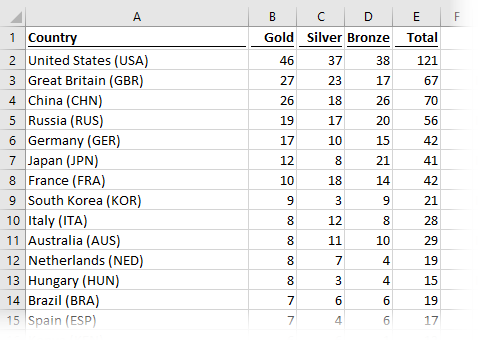
The screenshot above shows the 2016 Olympic Games medal table. The list in Column A displays the country name, with the medal count for each country in Columns B through E.

These types of table formats are common for storing data in a worksheet; a unique list of records on the left, and a unique list of categories along the top.

How could we use a formula to lookup the number of bronze, silver, gold, or total medals received by a single country? This is when you would turn to INDEX MATCH MATCH, as it is by far the simplest and most powerful method of performing a lookup based on rows and columns.

Applying the INDEX MATCH MATCH formula

To understand how this INDEX MATCH MATCH works, we will consider each function individually, then build-up to the combined formula.

MATCH

The MATCH function searches for an item in a list, then returns the relative position of the item within that list. Using our Olympic Games example, if we looked for Japan (JPN) from the country list in column A, it would return 6, as it is the 6th item in the list.

The syntax for the MATCH function is as follows:

=MATCH(lookup_value, lookup_array, [match_type])

• lookup_value: the value to match. It can be a number, text, logical value (i.e., true/false) or a reference to a cell containing a number, text, or logical value.
• lookup_array: the range of cells in which to search for the lookup_value.
• [match_type]: a value of 1, 0, or -1, which tells Excel how the lookup calculation should be performed. The square brackets indicate this argument is optional. However, if a value is omitted, Excel will assume the match_type should be 1. This is definitely not a safe assumption for Excel to be making, so always insert an argument, rather than letting the default apply.

The match_type is important, as it can affect the result of the calculation in unexpected ways.

• 1 = the function returns the largest value which is less than or equal to the lookup_value. To use this option, the lookup_array must be in ascending order.
• -1 = the function returns the smallest value which is greater than or equal to the lookup value. To use this option, the lookup_array must be in descending order.
• 0 = the function returns the first exact match found. For this option, the lookup_array can be in any order.

Example using the MATCH function

The screenshot below displays an example of using the MATCH function to find the position of a lookup_value.

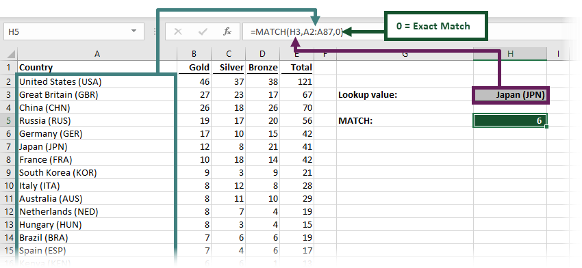
The formula in cell H5 is:

=MATCH(H3,A2:A87,0)

• H3 = Japan (JPN) – the lookup_value.
• A2:A87 = list of countries – the lookup_array
• 0 = an exact match – the match_type

The result in Cell H5 is 6. Japan (JPN) is the 6th country in the list, so the MATCH function returns 6.

Important note: The result returned is not the row number, but rather the nth row from the start of the lookup_array. 

MATCH works with rows or columns

The MATCH function works equally well with rows or columns. Using this same function across columns, we are also able to retrieve the position of the word ‘Bronze’.

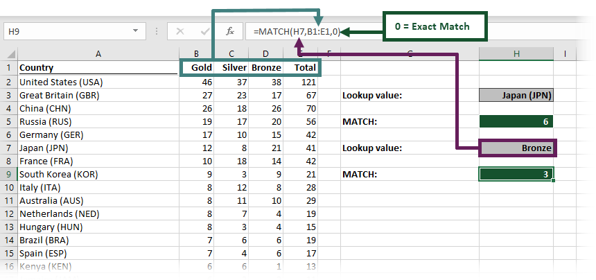
The formula in cell H9 is:

=MATCH(H7,B1:E1,0)

• H7 = Bronze – the lookup_value.
• B1:E1 = list of medals across the columns – the lookup_array
• 0 = an exact match – the match_type

The text string ‘Bronze’ matches with the 3rd column in the range B1 to E1, therefore the MATCH function returns 3 as the result.

Summary of the MATCH function

The image below contains a summary of the MATCH function.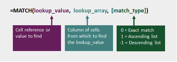

Find out more about the MATCH function in this article: MATCH function (support.office.com)
Microsoft recently released the XMATCH function, which you may have in your version of Excel. Find out more about the XMATCH function here: XMATCH function (support.office.com)

INDEX

The INDEX function returns the reference to a cell based on a given relative row or column position. It sounds much harder to understand than it is. For example, if INDEX were calculating the 7th cell within the range A5:A15, the result would be cell A11. Note, it would not be A12, as INDEX starts counting from 1. A5 is the 1st cell in the range, making A11 the 7th.

The INDEX function has two forms: (1) array form (2) reference form. We can see the two forms when we enter the formula using the insert function dialog.

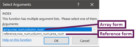
For this post, we will focus entirely on the array form, which is by far the most commonly used.

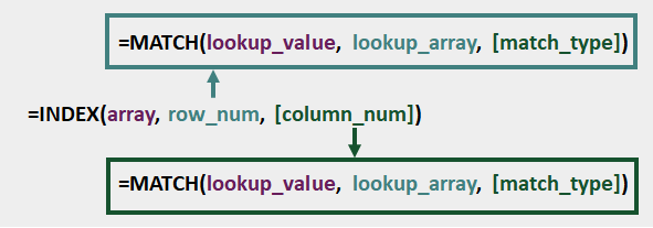
The syntax for the array form of the INDEX function is as follows:

=INDEX(array, row_num, [column_num])

• array – the range of cells from which to find the position
• row_num – the nth row position to locate in the array
• [column_num] – the nth column position to locate in the array. Within the INDEX function, this is an optional argument but is essential for the INDEX MATCH MATCH combination.

Example using the INDEX function

The screenshot below displays an example of using the INDEX function to find the result based on country and medal type.

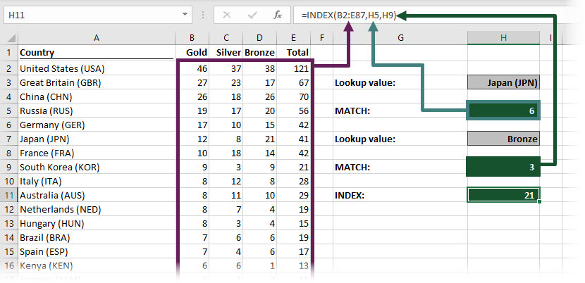
The formula in cell H11 is:

=INDEX(B2:E87,H5,H9)

• B2:E87 = the range of cells for the whole medal table – the array.
• H5 = 6 – the result from the first MATCH function – the row_num
• H9 = 3 – the result from the second MATCH function – the column_num

The 6th row and 3rd column in the range B2:E87 is cell D7. Since D7 contains the value 21, the result of the INDEX function is 21. The INDEX function’s ability to return a cell reference is an important feature, which we will consider later in this post.

Summary of the INDEX function

The image below contains a summary of the INDEX function.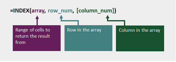

Find out more about the INDEX function in this article: INDEX function (support.office.com)

Nesting MATCH inside INDEX

The good news, is that whilst there are three separate functions at work here, we can place all the functions in a single formula.

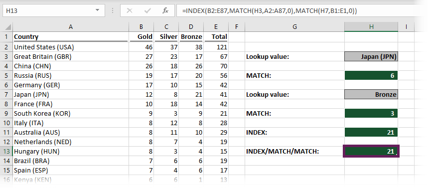
The formula in H13 is:

=INDEX(B2:E87,MATCH(H3,A2:A87,0),MATCH(H7,B1:E1,0))

For the row_num and column_num arguments in the INDEX functions we inserted the MATCH functions we created earlier.

It might have looked a bit scary, but now that we’ve built it up in stages, I hope you’ll agree that it’s not so bad after all.

Common errors

As there are three functions combined in a single formula, troubleshooting errors can be a bit tricky. But there are some common problems which you should check for first.

lookup_value not found in the lookup_array

The most common error with the MATCH function is #N/A. This can occur where:

• the match_type is 0 and the lookup_value is not found in the lookup_array
• the first value in the lookup_array is lower than the lookup_value when using a match_type of -1
•  the first value in the lookup_array is higher than the lookup_value when using a match_type of 1
• the lookup_value or lookup_array contains values that are formatted as text, rather than numbers
• the lookup_value or lookup_array contains leading or trailing spaces. Some characters are unseen to the human eye (try using the TRIM function to remove the spaces).

Incorrect or missing match_type in the MATCH function

Using the wrong match_type, or excluding the match_type from the MATCH function can cause calculation errors. These are the worst types of errors as the formula may appear to return the correct result, but it’s not. Check your formula result manually a few times to make sure it is returning the right value.

The other likely outcome of this issue is the #N/A error (see above). This is much more useful as we know it’s an error.

MATCH lookup_array and INDEX array not the same size

A #REF! error can occur when a MATCH is found, but the INDEX array is not big enough to include that row. For example, if there are 10 rows in the MATCH lookup_array, but only 5 rows in the INDEX array, a #REF! error will be returned for any MATCH in the 6th to 10th position.

If you still can’t find the cause of the error

If, after trying these options, you are still unable to find the cause of the error, try building up the formula from the three individual functions, as shown in the examples above.

INDEX MATCH MATCH with Tables

The best method for managing worksheet data is in an Excel table.

Tables introduced a new way of referencing cells and ranges. Rather than using the standard A1 notation, they use structured referencing, which refers to column names, rather than individual cells.  INDEX MATCH MATCH is happy to work with tables too.

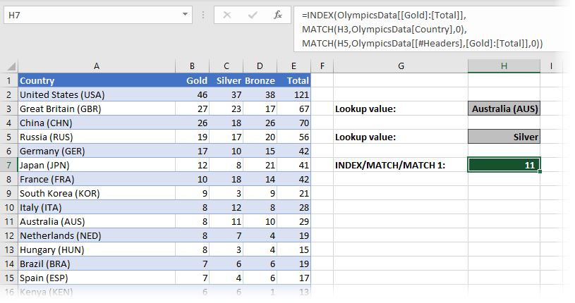
The image above comes from the Example 2 tab of the example file. The formula in cell H7 is: (for readability, it has been split into three lines below).

=INDEX(OlympicsData[[Gold]:[Total]],
MATCH(H3,OlympicsData[Country],0),
MATCH(H5,OlympicsData[[#Headers],[Gold]:[Total]],0))

• OlympicsData[[Gold]:[Total]] = the columns in the table from which to return the result – the array.
• H3 = Australia (AUS) – the lookup_value to find in the rows
• OlympicsData[Country] = list of countries – the lookup_array for the rows
• H5 = Silver – the lookup_value to find in the columns
• OlympicsData[[#Headers],[Gold]:[Total]] = the headers in the columns from Gold to Total. – the lookup_array for the column

The MATCH functions will find the result on the 10th row and 2nd column, which leads to cell C11. Since C11 contains the value 11, the result of the INDEX MATCH MATCH is 11.

Why tables work so well with INDEX MATCH MATCH?

Structured referencing is one of the best things about Excel tables. We know the range A2:A87 contains cells which list the countries, but we only know this by looking at the data. If we just looked at the formula, without paying any attention to the data, we would have no clue as to what is included in those cells.

With structured referencing, (assuming we have used sensible names for the table and columns), the range is referred to using the table and column name, such as OlympicsData[Country]. Without even looking at the data, we can take a pretty good guess as to what might be included in that range. Compare the table version of the formula to the standard version of the formula. I’m sure you’ll agree that the table version is much easier to understand.

But wait… there is another fantastic feature of tables. Any data added to the bottom of an Excel table is automatically included within the range. Try it out for yourself, add some data into cell A88 of the Example 2 worksheet. The table will automatically expand, as will the formula. Meaning there is no need to change the formula, it still works.

Next, try entering data in cell A88 of the Example 1 worksheet, the formulas do not update, therefore to incorporate that extra row we would need to change the INDEX and MATCH functions accordingly, which is just a waste of your time.

It is well worth investing time in learning how to use tables in Excel.

Advanced INDEX MATCH MATCH uses

Many Excel experts will advocate INDEX MATCH as better than VLOOKUP. Equally, INDEX MATCH MATCH is better than VLOOKUP MATCH, or other function combinations for two-dimension lookups. It allows us to use the following advanced techniques, creating greater flexibility in our Excel workbooks.

Return a value above, below, left or right of the matched value

INDEX MATCH MATCH can find the result above, below, left or right of the matched value.

Use the Example 3 tab from the example workbook. We will use a formula to find out which country is above Japan (JPN) in the medal table and how many gold medals they received.

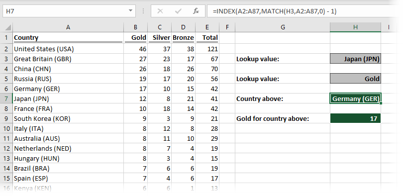
The formula in H7 subtracts 1 from the result of the MATCH function; then, INDEX finds the country name.

=INDEX(A2:A87,MATCH(H3,A2:A87,0) - 1)

As you can see by checking the table, the country above Japan (JPN) is Germany (GER), which is the result of the formula.

The formula in H9 builds on this to find the number of gold medals the country above received.

=INDEX(B2:E87,MATCH(H3,A2:A87,0) - 1,MATCH(H5,B1:E1,0))

Using the same method of subtracting 1 from the result of the MATCH function, we can calculate that the country above Japan (JPN) received 17 gold medals.

Return the cell address of the matched value

The INDEX function is magic, as it returns the cell address, rather than just the value in the cell.

Following on from our previous example, how do we know which cell the result comes from? (i.e., which cell is showing Germany’s gold medals?)

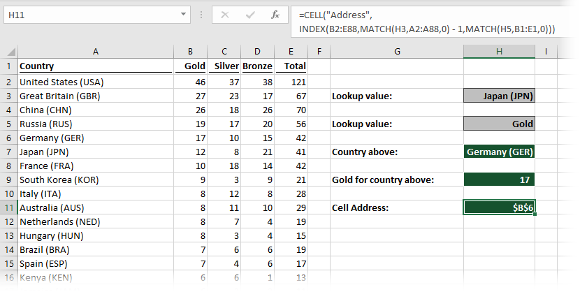
The formula in H11 uses the CELL function to return the address:

=CELL("address",INDEX(B2:E87,MATCH(H3,A2:A87,0) - 1,MATCH(H5,B1:E1,0)))

If we try wrapping VLOOKUP in the CELL function, it won’t work. VLOOKUP returns the cell value, rather than the cell reference This is the magic of INDEX 🙂

Create a dynamic range

As we have seen in the example above, the INDEX function returns a cell reference; therefore, we can create a dynamic range.

A range in Excel can be written as any two cells references separated by a colon. For example, B2: D4 is the range from cell B2 to cell D4. However, rather than using the cell reference, we can use a function that returns a cell reference.

Look at the formula below:

=SUM(B2 : INDEX (B2:F8,3,3))

The INDEX function calculates to cell D4. This is equivalent to:

=SUM(B2 : D4)

Now we’ve established the concept, turn to the Example 4 tab.

Let’s say we wanted to know how many Gold and Silver medals were won by all the countries from China (CHN) to Italy (ITA).

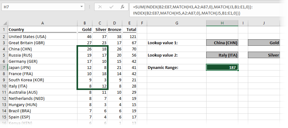
The formula in cell H7 is:

=SUM(INDEX(B2:E87,MATCH(H3,A2:A87,0),MATCH(J3,B1:E1,0)): 
INDEX(B2:E87,MATCH(H5,A2:A87,0),MATCH(J5,B1:E1,0)))

This is a standard SUM function, where the SUM range based on the results of the two INDEX functions. Did you notice the use of the colon ( : ) between the two INDEX functions, it is this which turns to two calculations into a range.

That long formula calculates down to the following:

=SUM(B3:C10)

Pretty amazing stuff, right?

Array formula to match multiple criteria in rows and/or columns

In the Example 5 tab, the 2012 Olympic Games medal table has now been added to the 2016 data, with a year column added to differentiate between the two. Our country list is no longer unique; each name can appear twice, once in 2012 and once in 2016.

When combining the country name with the year, we can still generate a unique reference again. We could use a helper column, but instead, we will use an array formula.

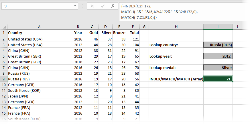
The formula in cell I9 is:

={INDEX(C2:F172,
MATCH(I3&"-"&I5,A2:A172&"-"&B2:B172,0),
MATCH(I7,C1:F1,0))}

Check the table for yourself, Russia received 21 silver medals in 2012.

The magic line of the formula is the second line. The lookup_value in the first MATCH function has been combined with a hyphen in between as a spacer character. The lookup_array has also been joined with a hyphen as a spacer character. This method turns the formula into a special type of formula known as an array formula.

Array formulas cannot be entered in the usual way (unless you have a dynamic array enabled version of Excel, see below). The curly braces at the start ( { ) and the end ( } ) are not part of the formula – don’t enter these into the formula bar. The curly braces are added by automatically by Excel when pressing Ctrl + Shift + Enter.

It is possible to use multiple criteria in the column headings too. This means INDEX MATCH MATCH can lookup a value from multiple criteria in the rows and/or columns.

INDEX MATCH MATCH with dynamic arrays

Dynamic arrays are the new way for Excel to return formula results. They were announced by Microsoft in September 2018, and are slowly being rolled out across different versions of Excel.

If you have a dynamic array enabled version of Excel, it is not necessary to press Ctrl + Shift + Enter to enter the INDEX MATCH MATCH formula in the example above. Excel will understand the formula and calculate the result.

However, if you do not have dynamic arrays in your version of Excel, it will display the #VALUE! error.

Anybody receiving your Excel workbook will also need the dynamic array version, so be careful where you use them. Probably best to stick with Ctrl + Shift + Enter until you know everybody who will view the file has a dynamic array enabled version.

Double XLOOKUP as an alternative

Microsoft has recently announced a new function called XLOOKUP, it will be available in newer builds of Excel. XLOOKUP has the advantages of INDEX MATCH, but with the simplicity of VLOOKUP.

We can nest an XLOOKUP within another XLOOKUP to achieve the equivalent result of INDEX MATCH MATCH. Sounds great, doesn’t it. However, at the time of writing (November 2019) I estimate it will be over 3 years before enough people have a compatible version to be able to use it reliably. Keep an eye out, as it is coming 🙂

Find out more about the XLOOKUP function in this article: XLOOKUP function (support.office.com)

Conclusion

While there are alternative ways to perform a two-dimensional lookup, currently none of them are as powerful as INDEX MATCH MATCH. This formula combination is so useful that it needs to be within your Excel toolkit.

Related Posts

• The real reason INDEX/MATCH is better than VLOOKUP
• How to VLOOKUP to the left
• How to change images based on cell values using INDEX/MATCH

---

What next?

Discover how you can automate your work with our Excel courses and tools.