How to VLOOKUP to the left

VLOOKUP is a very useful formula; most advanced Excel users still encounter situations where it would be a suitable solution. But a basic VLOOKUP has one major flaw; it cannot lookup a value to the left. The value being looked up must always be in the first column and the value returned must always be to the right. But data is not always provided like that, sometimes the data you wish to lookup is on the left – so what can you do?

I’ve got three options for you.

Create a duplicate column
Use the INDEX/MATCH functions
Use the VLOOKUP & CHOOSE functions together

The examples below use the following table:

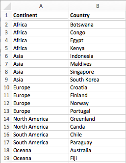
This is a very simple example with countries (Column B) and the continents they are in (Column A). The challenge is how do we find out the name of a continent based on the country name?

Option 1 – Create a duplicate column

This first option is not sophisticated and would make some Excel users shake their heads in disgust. But we could just duplicate Column A by copying it into Column C, then do a standard VLOOKUP. This solution would work perfectly well.

=VLOOKUP("Indonesia",B2:C19,2,FALSE)

This formula would return Asia as the result.

There are many ways in which this is not best practice, but sometimes we just do not need a complicated solution. In these circumstances this solution will work perfectly well.

Option 2 – Use the INDEX/MATCH functions

We can use the INDEX/MATCH functions. This is a combination of two separate functions, INDEX and MATCH. Let’s briefly look at each of these.

MATCH

The MATCH function will return a number indicating where in a list a specific value has been found. So, if we were to use a MATCH formula to find Indonesia in Cells B2-B19, it would return 5, as it is the 5th row in that range.

The format of the match formula is:

=MATCH(lookup_value, lookup_array, match_type)

The MATCH function is similar to VLOOKUP, but it does not require a column index number. It will only lookup in the list of cells contained in the lookup-array and will only return the position number.

MATCH has the match_type criteria, this is similar to VLOOKUP. We will want to use 0 in most circumstances to create an exact match.

INDEX

The INDEX formula returns a cell value based on the position number of a given range.

Having used MATCH to find that Indonesia is in the 5th row, we can use the INDEX formula to find the 5th item in the range.

=INDEX(A2:A19,5)

The INDEX formula would return Asia as a result.

Combining INDEX and MATCH

By combining INDEX and MATCH it is equivalent to a VLOOKUP that can lookup to the right or the left.

It is possible to combine INDEX/MATCH into a single formula; it is not necessary to calculate the functions in separate columns. Using our example, the full formula would be as follows:

=INDEX(A2:A19,MATCH("Indonesia",B2:B19,0))

If this is your first introduction to INDEX/MATCH I recommend you take time to learn more about how it works, as it is a very powerful formula combination, which can do much, much more than just replace VLOOKUP.

Option 3 – Use the VLOOKUP & CHOOSE functions together

This is by far the most complicated option, and the hardest to understand. But when combined with the CHOOSE function it is possible for VLOOKUP to look in any direction. The combined VLOOKUP and CHOOSE formula would look like this:

=VLOOKUP("Indonesia",CHOOSE({1,2},B2:B19,A2:A19),2,FALSE)

Let’s break down the CHOOSE function to understand what is happening:

=VLOOKUP("Indonesia",CHOOSE({1,2},B2:B19,A2:A19),2,FALSE)

The CHOOSE function in this situation is defining in which column is which. The numbers in the {} represent the column numbers and the ranges after the {} represent the cell ranges to which they relate. The red highlighted sections below shows that column 1 is defined as cells B2-B19.

=VLOOKUP("Indonesia",CHOOSE({1,2},B2:B19,A2:A19),2,FALSE)

The red highlighted sections below now show that column 2 is defined as cells A2-A19.

=VLOOKUP("Indonesia",CHOOSE({1,2},B2:B19,A2:A19),2,FALSE)

We can add as many columns as we like, but each number within the {} must have a corresponding range within the CHOOSE formula. Also, the numbers within the {} must be sequential. As an example, if we had 3 columns we could set out our formula as follows:

=VLOOKUP([lookup_value],CHOOSE({1,2,3},[lookup_range1],[lookup_range2],
[lookup_range_3]),3,FALSE)

Conclusion

There are many ways to achieve a lookup to the left. Depending on your Excel skill level and the complexity of your situation you can pick a solution which will work for you. Many Excel users believe that VLOOKUP cannot lookup to the left, but now you know that when combined with the CHOOSE function that it is possible.

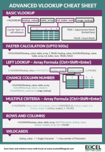
Download the Advanced VLOOKUP Cheat Sheet

Download the Advanced VLOOKUP Cheat Sheet. It includes most of the tips and tricks we’ve covered in this series, including faster calculations, multiple criteria, left lookup and much more.

Please download it and pin it up at work, you can even forward it onto your friends and co-workers.