Change number format based on a cell value in Excel

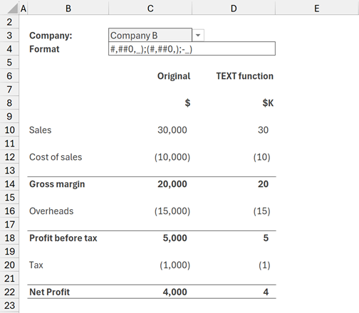
You’ve built an amazing dynamic report; a user selects a business unit to view, and everything updates automatically – it’s beautiful. The only issue is that Company A has sales of $30,000,000, Company B has sales of $30,000.

Displaying values in 1 decimal place millions makes sense for Company A. $30,000,000 becomes $30.0m. But it does not make sense for Company B. $30,000 becomes $0.0m.

The companies have different levels of significance. How can we format numbers so they work with either company?

In this post we look at 2 techniques.

Table of Contents

• Introduction to number formatting
• Option 1 – Use the TEXT function
• Option 2 – Conditional Formatting
• Conclusion

Watch the video

Watch on YouTube

Introduction to number formatting

Number formatting is a text string that tells Excel how to display a number. It doesn’t change the number itself, only how it looks.

We will not go into detail about number formats in this post. If you need to know more check out this post: Excel number formats for accounting & finance you NEED to know

Number formats are separated into 4 sections, all separated by semicolons.

[display of positive values] ; [display of negative values] ; [display of zero values] ; [display of text values]

We can format each section so that positive, negative, zero, and text values all display exactly as we want.

These number formats can include special characters which help to apply the desired formatting.

• # (hash) represents an optional digit. If a number is required it will display, if not, nothing displays.
• 0 (zero) represents a forced digit. Even if there is no number, a zero is still displayed. 
• , (comma) at the end of the number format forces the value to be divided by 1,000. Two commas means it is divided by 1,000,000.
• , (comma) between # or 0 indicates the thousand separator character,
• . (period) indicates where to place the decimal point.

Note: Based on regional settings, some characters may be different for you.

For this example, we have two number formats, which change depending on the value.

• If the sales value is less than 1,000,000, the number format is: #,##0,_);(#,##0,);-,_)
• If the sales value is 1,000,000, or greater the number format is: #,##0.0,,_);(#,##0.0,,);-,,_)

Now that we have a basic understanding of number formats, let’s examine how to apply them.

Option 1 – Use the TEXT function

The number formatting codes displayed above can be used within the TEXT function.

For this first example, the number formats are contained in a Table called Formats.

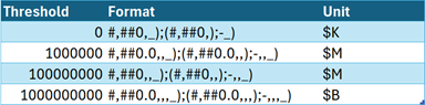
To retrieve the format code, we lookup the Threshold using the Sales value.

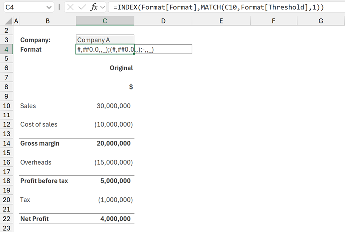
The formula in cell C4 is:

=INDEX(Format[Format],MATCH(C10,Format[Threshold],1))

This calculation uses an approximate match to return the closest value below the lookup value.

In the screenshot, cell C10 has a value of 30,000,000. The closest value below 30,000,000 is 1,000,000. Therefore the format returned is: #,##0.0,,_);(#,##0.0,,);-,,_)

We can apply format code using the TEXT function.

TEXT has two arguments:

• Value: the number to format.
• Format_text: the format to apply.

Using this, we can format any value to appear as we wish.

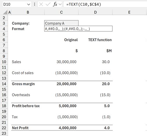
The formula in cell D10 is:

=TEXT(C10,$C$4)

This formula displays the value in C10 using the number format in cell C4.

The formula has been copied in D12, D14, D16, D18, D20 and D22.

When the values change to Company B, the formats update and apply the new number format.

It is important to realize the values are now text which looks like numbers. Therefore, we cannot calculate using these values.

To make this method work in the real world, we would need to:

• Calculate the actual values in a separate workings area.
• Display the values using the TEXT function on the face of the report.

Option 2 – Conditional Formatting

The second method uses conditional formatting. It takes a few more steps to apply, but we can continue to use the values as numbers.

Select the numbers in cells E10:E22.

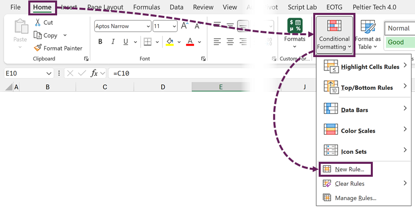
Click Home > Conditional Formatting > New Rule…

First, let’s set up the conditional format where the value is greater than or equal to 0.

Click use formula to determine which cells to format.

Enter the following formula:

=ABS($E$10)>=0

ABS calculates the absolute value for E10. Where it is greater than or equal to 0 the conditional formatting applies.

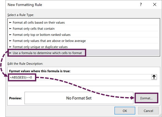
Click Format…

In the Format Cells window, select the Number > Custom

In the type box, enter the required number format. In our example, we are using:

#,##0,_);(#,##0,);-_)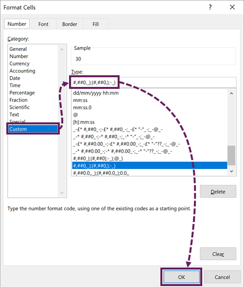

Click OK.

Repeat the process for values greater than 1,000,000. The number format applied in the example is:

#,##0.0,,_);(#,##0.0,,);-,,_)

You might be thinking – 30,000,000 is greater than 0 and greater than 1,000,000, so which number format applies?

Click Home > Conditional Formatting > Manage Rules… to view the rules.

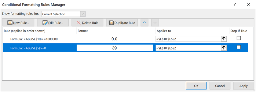
The format applied is based on the last format in the list where the formula evaluates to TRUE.

To apply the format based on the first condition, check the Stop If True box for each format.

The numbers now display different formats depending on the value. The values are still numbers, and we can calculate using those numbers.

The drawbacks of this method are:

• Need to create a separate conditional format for each threshold.
• If there is a lot of conditional formatting it can have performance issues.

Conclusion

In this post, we’ve seen two ways to apply number formatting based on a cell value. This ensures that we can apply a suitable level of display significance to values regardless of the underlying value.

Related Posts:

• How to create dynamic text in Excel (TEXT + Number Formats)
• Excel number formats for accounting & finance you NEED to know

---

What next?

Discover how you can automate your work with our Excel courses and tools.

---

What next?

Discover how you can automate your work with our Excel courses and tools.