Cell ranges: 99% of users don’t know this

I have never been taught how to use cell ranges in Excel; I doubt you have either. They are just too basic for anybody to teach, right? Select some cells, and there is a : (colon) symbol placed between the start and end cells. Maybe we could throw in a few $ (dollar signs) to fix the position of a cell reference. It’s hardly rocket science.

For most Excel users, that is everything they know about ranges, and everything they think they need to know. But that’s just the starting point; there is much more to uncover.

Ranges are the building blocks of Excel, so let’s ensure we understand how to use them correctly.

This post uncovers the methods for working with ranges that every Excel user should know.

Table of Contents

• Range operators
• Range operator
• Union operator
• Intersection operator
• Order of precedence
• Functions that return cell ranges
• CHOOSE
• IF
• IFS
• INDEX
• INDIRECT
• OFFSET
• SWITCH
• XLOOKUP
• Other operators and syntax
• Absolute marker ($)
• Spill operator
• Implicit intersection operator
• Conclusion

Range operators

Range operators are the special characters we place between individual cell references to create a range.

There are 3 operators:

• Range operator: Creates a single 4-sided range area.
• Union operator: Creates a range by joining two or more ranges together.
• Intersection operator: The range shared by two or more ranges.

Let’s start by understanding these operators.

Range operator

The range operator is the : (colon) symbol. We see this symbol when selecting a range using the mouse or keyboard shortcuts.

Since this is the operator that most Excel users know, we won’t spend too long on this one.

Here is an example of the range operator in use.

=SUM(B2:D4)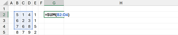

Result: 42

The range operator combines all the cells (including the two cells in the reference) into a single 4-sided range.

Nothing too complex here.

Once joined with the union operator or intersection operator, the range operator becomes even more powerful.

Union operator

The union operator is the , (comma) symbol. 

You may have seen the comma used in the in the following situation:

=SUM(B2,D3,C4)

Result: 14

However, in this scenario, the comma is not the union operator but the argument separator.

Within a function, arguments are separated by a comma. For example, the SUM function can include 255 items to aggregate, each separated by a comma. In this example, we provided SUM with 3 arguments; we have not used the union operator.

We must include additional brackets to use the union operator within a function, so Excel knows not to treat the comma as an argument separator.

=SUM((B2,D3,C4))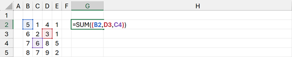

Result: 14

In the example, the calculation returns the same result, but that will not always be the case.

It may appear we are simply listing cells. While that is how we list items in a sentence, or in Power Query, that’s not how cell references work. 

The calculation combines the individual ranges into a single range before executing.

The power of the union operator is seen when combined with the range operator. Look at the image below; we are summing the values in the two ranges as if there were a single range.

=SUM(B2:D2,C4:E4)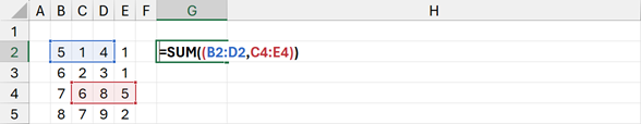

Result: 29

Intersection operator

The Intersection operator is the (space) character.

The intersection operator returns the range shared by two or more ranges.

Look at the example below:

=SUM(B3:E4 C2:D5)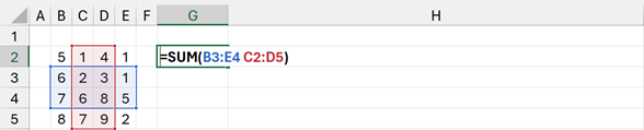

Result: 19

The formula in cell G2 calculates the range where the two other ranges intersect (i.e., the area where the ranges cross over) at cells C3:D4.

When using the intersection operator, we can include multiple ranges. For example, B3:E4 C2:D5 D2:E4 would be acceptable syntax for 3 ranges, returning D3:D4.

Order of precedence

Now, what happens if we mix operators in a single range? How does that impact calculation?

Within Excel’s calculation rules, there is a calculation order already set.

1. Range operator
2. Intersection operator
3. Union operator

Let’s take a look at 3 examples to see this in operation.

Example #1

Look at the following, what will the result be?

=SUM((B3:E3 C2:C5,D4))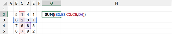

1. B3:E3 and C2:C5 calculate first
2. Next, the intersection between the two ranges calculates, leaving just cell C3
3. The union operator evaluates, giving a range of C3,D4.
4. Therefore, the final calculation is =SUM((C3,D4))

Result: 10

Example #2

If we want to force the calculation order, we can use brackets (just like with any nested functions in Excel).

=SUM((B3:E3 (C2:C5,D4)))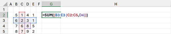

1. The brackets evaluate first:
   • Range operator C2:C5 is calculated.
   • Next, as there is no intersection in the brackets, the union operator evaluates, leaving the range C2:C5,D4.
2. Next, the intersection is evaluated. The only cell that intersects between B3:E3 and C2:C5,D4 is C3.
3. Therefore, the final calculation is =SUM((C3)).

Result: 2

Example #3

Take a look at the following example; what will that calculate? This is a tricky one.

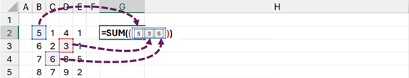
=SUM(B2:(D3,C4))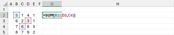

1. Brackets calculate first:
   • There is only a union operator within the brackets, so this evaluates as D3,C4.
2. The only operator remaining is the range operator. The purpose of the range operator is to create a single 4-sided range. So, Excel creates a range that encompasses all 3 ranges. This can only be B2:D4.
3. This leads to the final calculation of =SUM(B2:D4).

Result: 42

Even though D4 was not one of the cells in the formula, it is required to include D3 and C4.

If you tell me this didn’t blow your mind, I won’t believe you.

Functions that return cell ranges

One of the challenges of working with ranges, is when we don’t know the address of the cells to include in the formula. This occurs when we need a calculation to determine the range to use; known as a dynamic range.

Thankfully, there are several functions we can use to calculate a range address.

Instead of referencing a cell, we can include a formula that calculates the range.

Let’s use a simple example:

=SUM(B2:IF(A1=1,D4,D10))

• When the value in cell A1 is 1, IF returns a cell reference of D4. This creates a range of =SUM(B2:D4).
• When the value in cell A1 is not 1, IF returns a cell reference of D10. This creates a formula of =SUM(B2:D10).

So, depending on the value in cell A1, the range changes in size.

The syntax may seem confusing initially, as there is a formula directly after the colon. Excel calculates the formula first, then returns the cell address to create the range for the subsequent formula.

This creates enormous flexibility because we can create ranges on the fly inside formulas.

The functions that return ranges are: CHOOSE, IF, IFS, INDEX, INDIRECT, OFFSET, SWITCH, and XLOOKUP. Let’s take a brief look at each of these functions.

To know more about these functions, check out Alan Murray’s book, Advanced Excel Formulas.

CHOOSE

The CHOOSE function can select different cell ranges based on an index number. 

Let’s look at an example of using CHOOSE to select a range to return.

=SUM(CHOOSE(G4,B2:B5,C2:C5,D2:D5,E2:E5))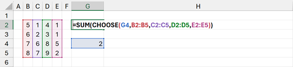

The first argument of the CHOOSE function is the index number. The remaining arguments are a list of possible results.

Using the example above:

• The index number in cell G4 is 2.
• Therefore, the 2nd item in the remaining arguments is returned, which is cells C2:C5.
• The formula above becomes =SUM(C2:C5).

Result: 16

IF

The IF function can return a range based on conditional logic.

The following is an example of using IF as one side of the range operator.

=SUM(C2:IF(G4=2,C5,D5))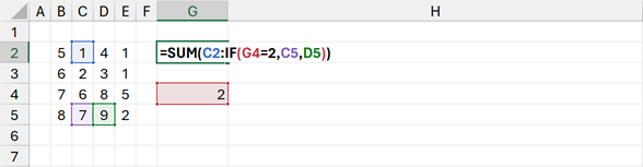

Using the example above:

• The IF evaluates to TRUE because cell G4 equals 2.
• The range created is C2:C5.
• The formula above becomes =SUM(C2:C5).

Result: 16

IFS

The IFS function can calculate a range based on a series of logic tests and returns the first value that evaluates to TRUE.

The following uses IFS to return an entire range into the SUM function.

=SUM(IFS(G4=1,B2:B5,G4=2,C2:C5,G4=3,D2:D5,G4=4,E2:E5))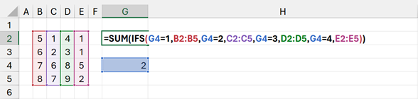

• Cell G4 is equal to 2; therefore, the range C2:C5 is returned.
• The formula above becomes =SUM(C2:C5).

Result: 16

INDEX

The INDEX function can return the nth row and nth column from a range as a cell reference.

The following example uses INDEX as one side of the range operator.

=SUM(C2:INDEX(B2:E5,G4,G5))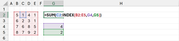

• Based on range B2:E5, INDEX returns the 4th row (cell G4) and 2nd column (cell G5). Which calculates as C5.
• The range operator creates a range of C2:C5.
• The formula above becomes =SUM(C2:C5).

Result: 16

With the INDEX function, if the row or column value is zero or blank, the value returned is the entire row or column.

=SUM(INDEX(B2:E5,G4,G5))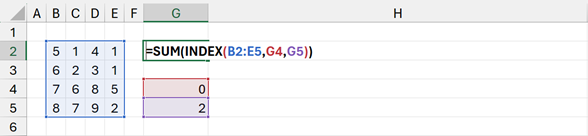

• Based on range B2:E5, INDEX returns all the rows (0 in cell G4) from the 2nd column (cell G5). Which calculates as C2:C5
• The formula above becomes =SUM(C2:C5)

Result: 16

INDIRECT

INDIRECT converts a text string into a range or cell reference. 

Let’s take a look at an example using INDIRECT.

=SUM(C2:INDIRECT(G4))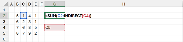

• INDIRECT(G4) converts the text value C5 into a range.
• The range created by the union operator is C2:C5.
• The formula above becomes =SUM(C2:C5).

Result: 16

OFFSET

The OFFSET function can create a range based on a cell position combined with width and height arguments.

Let’s take a look at an example.

=SUM(OFFSET(B2,G4,G5,G6,G7)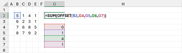

• The OFFSET function starts at cell B2 and then creates a range that is 0 rows down (G4), 1 column across (G5), 4 rows high (G6), 1 column wide (G7). This creates the range C2:C5.
• The formula above becomes =SUM(C2:C5).

Result: 16

SWITCH

The SWITCH function is a mixture between the CHOOSE and IFS functions. It can return a range based on matching the value in the expression argument.

In the following example, SWITCH returns a full range to the SUM function.

=SUM(SWITCH(G4,1,B2:B5,2,C2:C5,3,D2:D5,4,E2:E5))

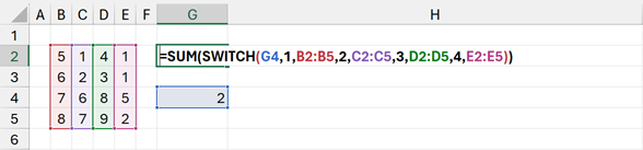
• The value in G4 is 2. The range following the value 2 in the argument list is C2:C5.
• The formula above becomes =SUM(C2:C5).

Result: 16

XLOOKUP

XLOOKUP looks up a value from a range and returns the corresponding cells from another range.

In the following example, we will keep it simple by using only the required arguments for the XLOOKUP function.

=SUM(C2:XLOOKUP(G4,B2:B5,C2:C5))

• XLOOKUP finds the value 8 (cell G4) from the range B2:B5 and returns the corresponding range from C2:C5. As 8 is the 4th cell in B2:B5, it returns the 4th cell in C2:C5, which is C5
• The range created by the union operator is C2:C5
• The formula above becomes =SUM(C2:C5)

Result: 16

Other operators and syntax

The range operators in the first section deal with basic range creation from standard cell references. But there are other operators we need to be aware of too.

• Absolute marker: For freezing cell references.
• Spill operator: For working with dynamic arrays.
• Intersection operator: For working with cell references in the same row or column.

Let’s take a look at each of these.

Absolute marker ($)

The absolute marker is the $ (dollar) symbol. This is a symbol that most users understand and are familiar with.

Where a $ symbol exists before a column letter or row number, that row or column becomes frozen when copying/pasting the formula to another location.

Where either the column or row is frozen, it is known as a mixed reference. When both the row and column are frozen, it is known as an absolute reference.

• Relative reference: A1
• Mixed references: $A1 or A$1
• Absolute reference: $A$1

After selecting a cell reference, pressing the F4 key cycles through the 4 options: $A$1, A$1, $A1, A1.

This $ symbol is ignored by Excel when it evaluates formulas; it is only used when copying or dragging formulas into other cells.

Mixing absolute, relative, and mixed references in a single range is permitted. For example, A1:$D$10, $E4 is valid syntax and contains relative, absolute, and mixed references.

Spill operator

The spill operator is the # (hash/pound) symbol. This symbol obtains the full range occupied for a dynamic array calculation.

In the example below, the UNIQUE function generates a list of unique values from the original source. The data could have an unknown number of unique values; therefore, the range filled by UNIQUE is of an unknown size.

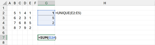
The formula in cell G2 is:

=UNIQUE(E2:E5)

The formula in cell G7 is:

=SUM(G2#)

G2# provides a way to reference a range returned by the formula in G2, no matter the number of rows or columns produced.

Implicit intersection operator

The implicit intersection operator is the @ (at) symbol. This symbol is used to return only the cell that exists in the same row or column as the formula that is referencing the range.

In the example below, the range C2:C5 is used in every formula. The @ symbol returns only the cell which exists in the same row.

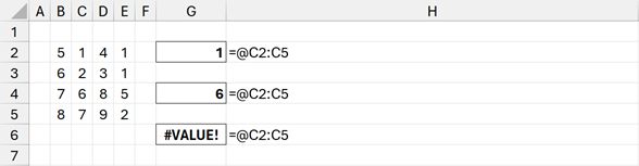
• Cell G2 returns the value in cell C2
• Cell G4 returns the value in cell C4
• Cell G6 returns the #VALUE! error as there are no values in C2:C5 that exist in the same row as the formula.

This approach works for both rows and columns.

Conclusion

You’re now an Excel Range ninja. You’ve got all the tools you need to create very powerful (yet simple) Excel models. The only limit now, is your creativity.

---

What next?

Discover how you can automate your work with our Excel courses and tools.